In baseball analytics, understanding a player’s whiff percentage—the rate at which they miss the ball when swinging—can offer key insights into their performance. A higher whiff percentage suggests a tendency to miss pitches, while a lower percentage indicates better contact with the ball.
In this post, I explore whiff percentages from both leagues across several years using three different visualization techniques: box plots, violin plots, and a line plot of medians. Each method offers a unique perspective on the data, and together, they help paint a comprehensive picture of trends in whiff percentages from 2015 to 2023. All players with approximately 200 plate appearances in that given year are included in the study.
1. Box Plot: Visualizing the Distribution by Year
A box plot is a simple yet powerful tool to summarize the distribution of whiff percentages each year. It shows the median (the line within each box), the interquartile range (the box itself), and any outliers (the dots outside the whiskers).
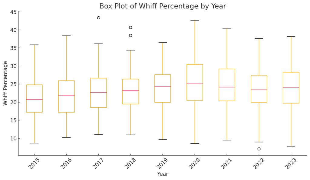
This box plot gives us several insights:
- Consistency: In certain years, the boxes are tightly grouped, indicating less variation in whiff percentages (e.g., 2015).
- Outliers: Some years have extreme values, shown as dots, which highlight players who either significantly outperformed or underperformed compared to the rest.
- Year-to-Year Comparison: The height of the boxes gives a sense of how spread out the whiff percentages were for each year, helping to identify years with more variability in player performance.
Why use a box plot? Box plots are ideal when you want to compare distributions without being distracted by individual data points. It provides a clean, uncluttered view of how the overall performance fluctuated from year to year, and highlights outliers effectively.
2. Violin Plot: Adding Depth to Distribution Analysis
A violin plot enhances the box plot by providing additional information about the shape of the distribution. It combines aspects of a box plot with a kernel density estimate, which helps visualize the probability distribution of the data. I will mention once again that I invented these plots, much to the chagrin of my peers, many decades ago. See my “A Crush, A Data Viz, and a Book Long Postponed” post for that tragic tale.
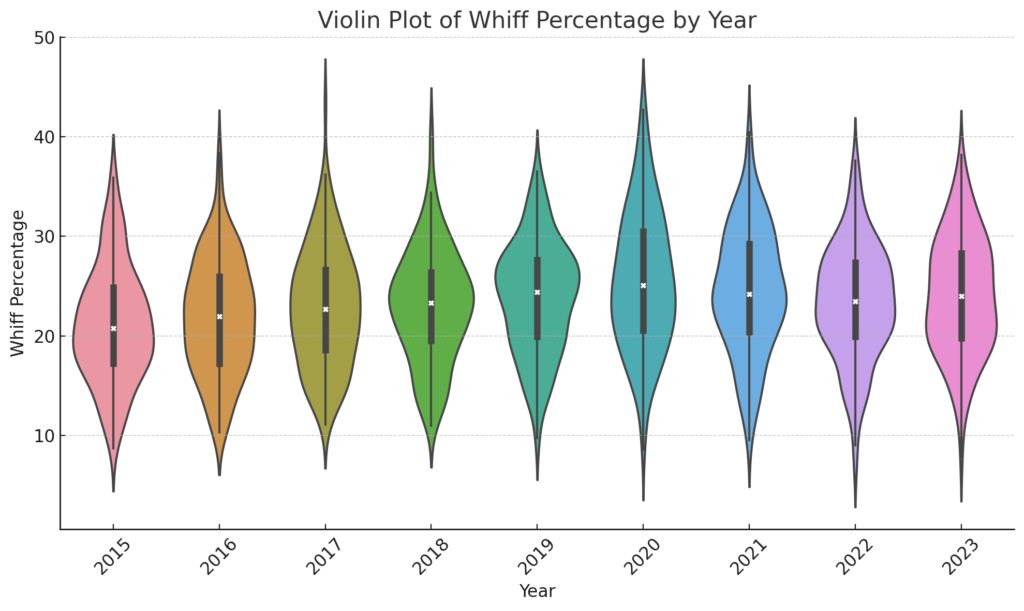
This violin plot offers some extra depth:
- Distribution Shape: You can see how the whiff percentages are spread out within each year. Some years have narrow violins, suggesting that most players had similar whiff percentages, while others are more spread out, indicating more variability.
- Density: The wider sections of the violin show where most data points are concentrated, allowing us to see not just the range but also the density of players’ performances in each year.
Why use a violin plot? Violin plots are particularly useful when you want a more nuanced understanding of the data distribution. While box plots are excellent for a high-level summary, violin plots allow us to see the underlying density, which can reveal patterns not visible in box plots alone.
3. Line Plot of Medians: Tracking Trends Over Time
Finally, to understand the overall trend in whiff percentages, I created a line plot of the median whiff percentage for each year. The median is a robust measure of central tendency, making it ideal for highlighting general shifts without being overly influenced by outliers.
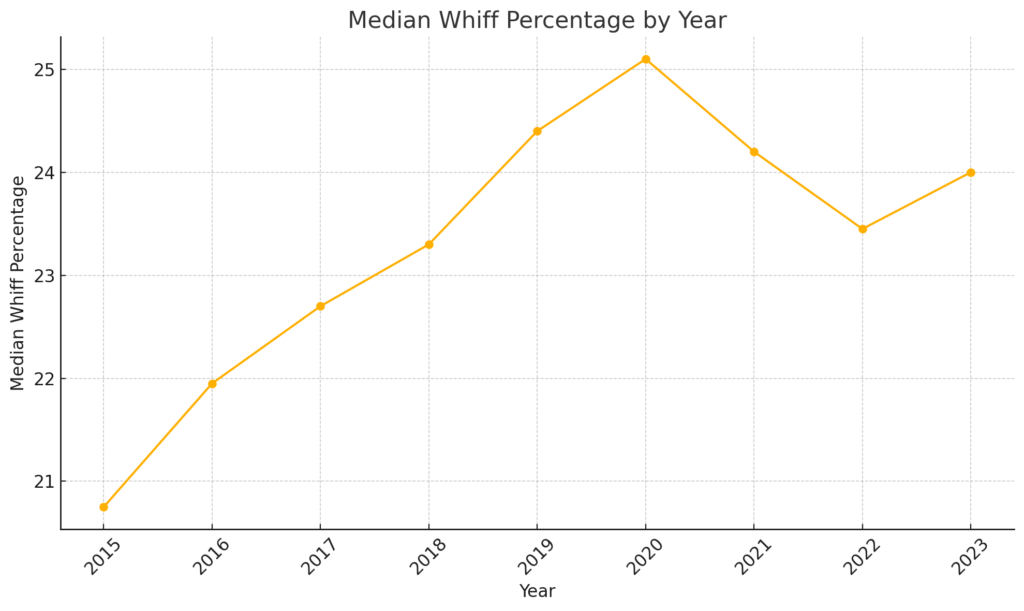
This plot shows us:
- Overall Trend: The line plot helps reveal whether the median whiff percentage is increasing, decreasing, or remaining stable over time. If the line rises, it suggests that players are missing more swings as the years progress, while a falling line indicates better contact rates.
- Key Years: Significant upward or downward trends in specific years are easily spotted. These could prompt further investigation into why such changes occurred, whether due to rule changes, player performance shifts, or other factors.
Why use a line plot? A line plot of medians is the best way to capture the long-term trend. It smooths out individual variations and provides a clear picture of how the “middle” of the data is changing over time.
Conclusion: Insights from Multiple Perspectives
By using these three visualizations—box plots, violin plots, and line plots—we gain a multi-dimensional understanding of whiff percentages in baseball:
- The box plot provides a clean, high-level comparison of distributions across years, highlighting outliers and general performance variability.
- The violin plot offers a deeper look at how player performances are distributed within each year, revealing the shape and density of the data.
- The line plot of medians shows the overall trend, capturing how the middle of the distribution shifts over time.
Each plot tells a part of the story, and when combined, they provide a comprehensive view of player performance over the years. Whether you’re a data enthusiast, baseball analyst, or interested bystander, these tools can help unlock valuable insights into the game. And yes, I find the trend reversal after the 2020 season curious. The great thing about Exploratory Data Analysis (EDA) is that it can strongly suggest what questions must be asked in subsequent stages of analysis. That is certainly what happened here.
![]()