Zeno’s Paradox: The Infinite Hidden Inside a Single Step

At first glance, Zeno’s paradox seems ridiculous.

Of course, Achilles catches the tortoise. Of course, an arrow moves through the air. Of course, I can walk across a room. Well, duh!

We know these things before anyone begins arguing. Motion is one of the most ordinary facts of experience. Every thrown ball, every running child, every falling leaf, every car moving down a road seems to refute Zeno before he even begins.

And yet the paradox remains.

That is what makes Zeno interesting. His argument does not stand because it leads us to believe that motion is impossible. It survives because it reveals something strange about the way we explain motion. Zeno takes an everyday event and slows it down until the ordinary becomes puzzling. He asks us to look not at the fact that something moves, but at what must be true for motion to be intelligible.

Before I can cross a room, I must first cross half the room. Before I can cross the remaining distance, I must cross half of that. Then half again. Then half again. The distances become smaller and smaller, but the number of required divisions seems to grow without end.

The paradox begins with a simple observation: A finite distance can be divided into infinitely many parts.

That is the unsettling idea at the heart of Zeno’s paradox. The problem is not that the room is too large. The problem is that even a small room appears to contain an infinite structure.

The question becomes: how can a person complete an infinite number of tasks in a finite amount of time?

The Dichotomy Paradox

One of Zeno’s most famous arguments is often called The Dichotomy Paradox. The word “dichotomy” means a division into two parts. In this paradox, every journey must be divided in half.

Suppose I want to walk from one side of a room to the other. To reach the far wall, I first need to reach the halfway point. Once I reach the halfway point, I still need to reach the halfway point of the remaining distance. Then I need to reach the next halfway point. And so on.

The sequence looks like this:

\frac{1}{2},\ \frac{1}{4},\ \frac{1}{8},\ \frac{1}{16},\ \frac{1}{32},\ldots

Each distance is smaller than the one before it. But there is no final term. No matter how many halfway points I cross, another halfway point remains.

That is the apparent trap. If every motion requires completing infinitely many sub-motions, then motion seems impossible. Before I can finish the journey, I must finish an infinite sequence of smaller journeys.

Yet I do finish the journey.

That tension is the paradox.

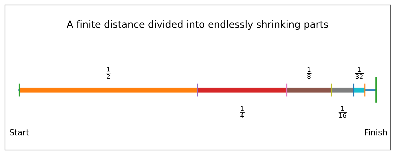
Figure 1. Divided Finite Distance.

Mathematically, the total distance can be written as an infinite series:

\frac{1}{2}+\frac{1}{4}+\frac{1}{8}+\frac{1}{16}+\cdots

At first, this looks like an endless accumulation. But modern mathematics gives us a clear answer:

\frac{1}{2}+\frac{1}{4}+\frac{1}{8}+\frac{1}{16}+\cdots = 1

More formally:

\sum_{n=1}^{\infty}\left(\frac{1}{2}\right)^n = 1

The infinite series has a finite sum.

This is the key mathematical insight. An infinite number of terms does not necessarily mean an infinite total. The terms can shrink quickly enough that their sum approaches a finite limit.

That is why the walker reaches the wall. The distances get smaller, and the times required to cross them also get smaller. The infinite sequence does not require infinite time.

Still, this answer should not make us dismiss Zeno too quickly. The modern solution is powerful, but it also shows why the paradox mattered in the first place. Zeno forced later thinkers to clarify the relationship between infinity, space, time, and motion.

He did not merely ask a trick question. He discovered a pressure point.

Achilles and the Tortoise

The most famous version of Zeno’s argument is Achilles and the tortoise.

Imagine Achilles, the great runner, racing against a tortoise. Since Achilles is much faster, the tortoise receives a head start. Once the race begins, Achilles quickly reaches the place where the tortoise started. But by that time, the tortoise has moved a little farther ahead.

Achilles then reaches that new position. But again, the tortoise has moved forward.

Achilles reaches the next position. The tortoise has moved again.

This continues indefinitely.

The distances shrink. The tortoise’s lead becomes smaller and smaller. But in Zeno’s framing, Achilles must first reach every previous position occupied by the tortoise. Since there are infinitely many such positions, it seems Achilles can never catch up.

Again, common sense rebels.

Of course Achilles catches the tortoise.

But Zeno is not really betting on the tortoise. He is asking whether motion can be explained if every interval contains infinitely many smaller intervals.

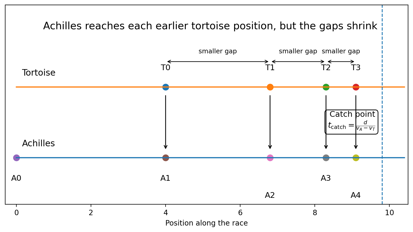
Figure 2. Race Diagram.

Let the tortoise begin with a head start of distance (d). Let Achilles run at velocity (vA), and let the tortoise move at velocity (vT). If Achilles is faster, then:

v_A > v_T

The time it takes Achilles to catch the tortoise is:

t_{\text{catch}} = \frac{d}{v_A - v_T}

This equation gives a finite answer. Achilles catches the tortoise when the initial head start has been eliminated by the difference between their speeds.

For example, suppose the tortoise starts 10 meters ahead. Achilles runs at 10 meters per second. The tortoise moves at 1 meter per second. Then:

t_{\text{catch}} = \frac{10}{10 - 1} t_{\text{catch}} = \frac{10}{9}

So Achilles catches the tortoise in about 1.11 seconds.

t_{\text{catch}} \approx 1.11\ \text{seconds}

The paradox dissolves mathematically. But it does not disappear philosophically. Zeno’s description of the race is not false in the ordinary sense. Achilles really does pass through the tortoise’s earlier positions. There really are infinitely many possible subdivisions of the race. What Zeno gets wrong is the assumption that infinitely many subdivisions require infinitely much time.

The modern answer depends on the idea of convergence.

The partial sums of a shrinking series approach a limit. For example:

S_n = \sum_{k=1}^{n}\left(\frac{1}{2}\right)^k

As (n) increases, (S_n) gets closer and closer to 1.

\lim_{n\to\infty} S_n = 1

This is the heart of the mathematical solution. The sequence has infinitely many steps, but the total distance is finite. The total time is finite too, assuming the motion is continuous, and the speed remains well-behaved.

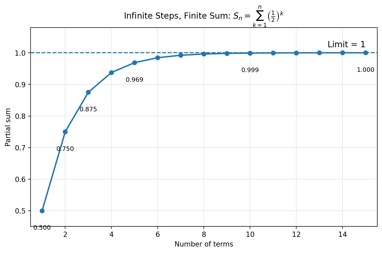
Figure 3. Infinite Steps

The Arrow Paradox

Zeno’s Arrow paradox attacks motion from another direction.

Imagine an arrow flying through the air. At any single instant, the arrow occupies a particular position. At that instant, it is exactly where it is. It is not yet at the next position, nor is it at the previous one.

So, Zeno asks, where is the motion?

If time is made of instants, and if the arrow is motionless at each instant, then how can motion arise from a collection of motionless moments?

This paradox is different from the Dichotomy and Achilles arguments. It is not mainly about an infinite sequence of distances. It is about time itself. If time is composed of indivisible instants, then motion becomes difficult to locate. At a single frozen instant, nothing appears to move.

A photograph captures this problem nicely. A photograph of a moving car does not show motion itself. It shows a car at a position. Motion appears only when we understand the position as part of a sequence.

Modern physics and calculus answer this by treating velocity not as a visible change inside a single instant, but as an instantaneous rate of change.

Average velocity is easy to understand:

v_{\text{avg}} = \frac{\Delta x}{\Delta t}

This says that average velocity equals change in position divided by change in time.

Instantaneous velocity is more subtle. It is defined as the limit of average velocity as the time interval becomes arbitrarily small:

v(t) = \lim_{\Delta t\to 0}\frac{x(t+\Delta t)-x(t)}{\Delta t}

The arrow does not need to move “inside” a frozen instant. Its motion is represented by the way its position changes over time. Velocity belongs to the structure of the function, not to a single isolated snapshot.

That is a powerful mathematical response. But again, Zeno has forced us to become more precise. He makes us distinguish between position and motion, between an instant and an interval, between a snapshot and a process.

The arrow paradox is not silly. It is a warning about confusing the parts of a description with the whole of reality.

Infinity as the Real Subject

The reason Zeno’s paradoxes endure is that they are not really about turtles, arrows, or people crossing rooms. They are about infinity.

There are at least two kinds of infinity at work here.

First, there is the infinity of division. A line segment can be divided in half, then half again, and so on. There is no obvious stopping point. This suggests that space may be infinitely divisible.

Second, there is the infinity of sequence. Once we begin listing the required steps, the list seems endless. First half the distance. Then half the remainder. Then half again.

Zeno’s genius was to combine these two ideas and turn them against motion.

If every finite act contains infinitely many parts, then how can any finite act be completed?

The modern answer is that infinitely many parts can form a finite whole. That answer now seems familiar because infinite series are part of standard mathematics. But the idea is far from obvious. It is one of the great achievements of mathematical thought.

A simple geometric series shows the point:

a + ar + ar^2 + ar^3 + \cdots = \frac{a}{1-r}

provided that:

|r| < 1

In the Dichotomy paradox, the first term is:

a = \frac{1}{2}

and the common ratio is:

r = \frac{1}{2}

So:

\frac{a}{1-r} = \frac{\frac{1}{2}}{1-\frac{1}{2}} \frac{\frac{1}{2}}{\frac{1}{2}} = 1

The infinite sum equals the finite distance.

This is why Zeno’s argument fails mathematically. But it fails in a revealing way. It shows that common sense alone is not enough. We needed a theory of limits to explain what everyday experience already knew.

The Difference Between Solving and Dismissing

It is tempting to say that calculus solved Zeno’s paradox and leave it there.

In one sense, that is true. The mathematics of limits gives a clean answer to the problem of infinite subdivision. Achilles catches the tortoise. The walker crosses the room. The arrow moves.

But there is a difference between solving a paradox and dismissing it.

A bad paradox depends on a cheap trick. Once the trick is exposed, nothing remains.

Zeno’s paradox is different. Even after the mathematical answer is given, the original problem remains intellectually productive. It continues to ask useful questions.

What is continuity?

What is an instant?

Is space made of points, or are points abstractions we impose on space?

Is time a flowing reality, or a coordinate in a mathematical model?

Does mathematics describe the world directly, or does it provide a structure that predicts the world?

These are not dead questions. They return in different forms in philosophy, physics, and mathematics. Zeno’s paradox survives because it sits near the boundary between lived experience and formal explanation.

We live in motion. But to explain motion, we must translate it into distance, time, velocity, sequence, and limit. Each translation clarifies something. Each translation also changes the problem.

The Paradox as a Lesson in Explanation

There is a deeper lesson here.

Zeno shows that an explanation can fail even when the reality being explained is obvious.

Motion happens. No serious person doubts that. But saying “motion happens” is not the same as explaining how motion is possible within a particular theory of space and time.

That distinction matters far beyond ancient philosophy.

In science, statistics, and history, we often begin with facts that seem obvious. A species changes. A river cuts a valley. A baseball player declines with age. A market rises or falls. A civilization expands. A population migrates.

But explanation requires structure. We need a model. We need assumptions. We need a way to connect observations to causes.

Zeno’s paradox reminds us that the structure of explanation can become unstable. Sometimes the model makes the obvious seem impossible. When that happens, the answer is not to reject experience immediately. It is to examine the assumptions inside the model.

That may be the real value of the paradox.

Zeno slows us down. He makes us ask what we mean by motion, distance, time, and completion. He takes a simple act and reveals the hidden machinery of thought inside it.

A single step across a room becomes a philosophical event.

Why the Paradox is Still Discussed

Zeno was wrong if his goal was to prove that motion is impossible.

But he was right that motion is stranger than it appears.

The paradox matters because it teaches humility. We should be careful when we assume that ordinary experience is simple. The simplest events often contain the deepest assumptions.

Walking across a room feels immediate. But when analyzed mathematically, it opens into infinity.

A runner passing a tortoise feels obvious. But when divided into successive positions, it becomes a puzzle about convergence.

An arrow flying through the air feels undeniable. But when frozen into instants, it becomes a question about time.

In each case, Zeno forces us to notice that reality and explanation are not identical. Reality happens. Explanation tries to account for how it happens. The gap between the two is where paradox lives.

The modern mathematical answer is beautiful:

\sum_{n=1}^{\infty}\left(\frac{1}{2}\right)^n = 1

An infinite process can have a finite limit.

But the philosophical lesson is just as important:

The world may move easily, but our concepts do not always move with it.

Conclusion: The Infinite in the Ordinary

Zeno’s paradox begins with common sense and ends with infinity.

That is why it remains powerful. It does not take us away from ordinary life. It takes ordinary life more seriously than we usually do.

A walk across the room becomes a question about infinite division. A race becomes a question about convergence. An arrow becomes a question about time, instants, and change.

The paradox is not really asking whether motion exists. It is asking whether our account of motion is coherent.

That is a much better question.

Achilles catches the tortoise. The arrow reaches the target. I cross the room.

But after Zeno, none of these things seems quite as simple as they did before.

The world still moves.

The mystery is that we can explain it at all.


Season-Level Validation: Do Third-Base Offensive Z-Scores Predict wRC+?

Season-Level Validation: Do Third-Base Offensive Z-Scores Predict wRC+?

Introduction

The first wRC+ validation study used a career-level FanGraphs export.

That study was useful. It showed that, among regular third basemen, average Model C offensive score per qualified season strongly predicted career wRC+. It also showed that traditional defense did not predict wRC+, which was exactly what we wanted from a negative-control test.

But the career-level study had one limitation.

wRC+ is fundamentally a season-level offensive rate statistic. Our offensive z-score system is also built season by season. So the cleanest validation test is not career score against career wRC+.

The cleanest test is:

Does a third baseman’s season-level offensive z-score predict his season-level wRC+?

This chapter answers that question.

The answer is yes.

Using the season-level FanGraphs export, the Model C offensive season score explains about 69 percent of the variation in season wRC+ among qualified third-base seasons.

R^2 = 0.692

The fitted model is:

wRC^+ = 101.47 + 5.86(\text{Model C Offensive Season Score})

That is a strong result.

Just as important, the traditional defensive score does not predict wRC+:

R^2 = 0.002

This is exactly the pattern the project needed.

Offensive z-scores predict offense.

Traditional defensive z-scores do not.

That means the Model C offensive score is not merely identifying generally good players. It is measuring offensive quality.

Data Used in the Season-Level Study

The FanGraphs season-level export included:

9,152 player-season rows through 2025
Season
Name
Team
PA
wRC+
PlayerId
MLBAMID

The broader third-base season dataset included:

3,188 qualified third-base seasons
Season range: 1880–2025

The merge was very strong:

Matched seasons: 3,163
Unmatched seasons: 25
Match rate: 99.2%

The remaining unmatched seasons were mostly older Negro Leagues or historical ID cases. The modern and post-integration major-league seasons matched very well.

This makes the season-level validation much cleaner than the first career-level wRC+ test.

Why Season-Level Validation Matters

The career-level wRC+ test asked whether accumulated third-base offensive separation was related to career offensive quality.

The season-level test is more direct.

It asks:

In a given season, does the offensive z-score model identify the same kind of offensive performance that wRC+ identifies?

This is a better test because both measures are season-specific.

The z-score model compares a third baseman to other third basemen in the same season. wRC+ compares a hitter’s offensive production to the league and park context of that season.

They are not the same statistic.

But they should be related.

If Model C is measuring offensive quality, high Model C scores should correspond to high wRC+ values.

That is what the data show.

The Model C Offensive Score

The Model C offensive score uses seven components:

OBP
ISO
BB/PA
SO/PA, inverted
Net SB/PA
R/PA
RBI/PA

Each component is converted into a same-position, same-season z-score.

The basic z-score formula is:

z = \frac{x - \mu}{\sigma}

Where:

x = \text{the player's value} \mu = \text{the same-position, same-season peer-group mean} \sigma = \text{the same-position, same-season peer-group standard deviation}

This is the central idea of the study.

Raw numbers ask how large a number is. Z-scores ask how far a player separated from his peer group.

Offensive Component Equations

On-base percentage is:

OBP = \frac{H + BB + HBP}{AB + BB + HBP + SF}

Slugging percentage is:

SLG = \frac{TB}{AB}

Isolated power is:

ISO = SLG - AVG

Walk rate is:

BB/PA = \frac{BB}{PA}

Strikeout rate is:

SO/PA = \frac{SO}{PA}

Net stolen bases are:

NetSB = SB - CS

Net stolen-base rate is:

NetSB/PA = \frac{SB - CS}{PA}

Run rate is:

R/PA = \frac{R}{PA}

RBI rate is:

RBI/PA = \frac{RBI}{PA}

The strikeout component is inverted because lower strikeout rates are better:

z_{\text{Low SO/PA}} = -\left( \frac{ (SO/PA)_i - \overline{(SO/PA)}_{\text{peer}} }{ s_{SO/PA,\text{peer}} } \right)

The full Model C offensive season score is:

\begin{aligned} \text{Season Score} &= z_{\text{OBP}} + z_{\text{ISO}} + z_{\text{BB/PA}} + z_{\text{Low SO/PA}} \\ &\quad + z_{\text{NetSB/PA}} + z_{\text{R/PA}} + z_{\text{RBI/PA}} \end{aligned}

This score measures offensive separation from same-season third-base peers.

Regression Framework

The main validation model is:

wRC^+_s = \alpha + \beta_1(\text{Model C Offensive Season Score}_s) + \varepsilon_s

Where:

wRC^+_s = \text{FanGraphs wRC+ for season } s \alpha = \text{intercept} \beta_1 = \text{slope for the offensive z-score} \varepsilon_s = \text{residual error}

The coefficient of determination is:

R^2 = 1 - \frac{ \sum_s \left( wRC^+_s - \widehat{wRC^+}_s \right)^2 }{ \sum_s \left( wRC^+_s - \overline{wRC^+} \right)^2 }

A higher value of R^2 means the model explains more of the variation in wRC+.

Main Season-Level Result

The fitted offense-only model is:

wRC^+ = 101.47 + 5.86(\text{Model C Offensive Season Score})

The result is:

R^2 = 0.692

This means the Model C offensive season score explains about 69.2 percent of the variation in season-level wRC+ among matched qualified third-base seasons.

That is a strong validation result.

The slope is also meaningful:

\beta_1 = 5.86

Each additional point of Model C offensive season score corresponds to about 5.86 additional points of wRC+.

For example, a player with an offensive score of 0 projects as:

wRC^+ = 101.47 + 5.86(0) wRC^+ = 101.47

A player with an offensive score of 5 projects as:

wRC^+ = 101.47 + 5.86(5) wRC^+ = 130.77

A player with an offensive score of 10 projects as:

wRC^+ = 101.47 + 5.86(10) wRC^+ = 160.11

This is exactly the pattern expected if Model C is capturing offensive dominance.

Figure 1: Model Comparison

Figure 1. How well season-level third-base metrics predict wRC+.

The first figure compares several models.

The offensive z-score model performs well:

R^2_{\text{Offensive z-score}} = 0.692

The traditional defensive score performs almost not at all:

R^2_{\text{Traditional Defense}} = 0.002

Adding traditional defense to offense does not meaningfully improve the result:

R^2_{\text{Offense + Defense}} = 0.692

Adding plate appearances produces only a tiny improvement:

R^2_{\text{Offense + PA}} = 0.695

The WAR_off benchmark is higher:

R^2_{\mathrm{WAR}_{\mathrm{off}}} = 0.846

That is expected. WAR_off is already a sophisticated offensive value measure. It is included only as a benchmark, not as a competing z-score model.

The important comparison is offense versus defense.

The offensive z-score score predicts wRC+ strongly. The defensive score does not.

Figure 2: Offensive Z-Score Versus wRC+

Figure 2. Season wRC+ versus Model C offensive season score among third basemen.

This figure shows the main relationship directly.

The x-axis is:

\text{Model C Offensive Season Score}

The y-axis is:

wRC^+

The fitted line is:

wRC^+ = 101.47 + 5.86x R^2 = 0.692

The pattern is clear.

High offensive z-score seasons generally produce high wRC+ seasons. Miguel Cabrera’s 2013 season, Chipper Jones’s 1999 season, Mike Schmidt’s 1980 and 1981 seasons, George Brett’s 1985 season, and Alex Rodriguez’s 2007 season all sit in the upper-right region.

That is exactly where they should be.

The plot also shows interesting residual cases. Some seasons have high wRC+ relative to their Model C score. Others have lower wRC+ than the z-score model predicts.

Those differences are not necessarily errors. They show that Model C and wRC+ measure offense from different angles.

Figure 3: Actual Versus Predicted wRC+

Figure 3. Actual versus predicted season wRC+ using the offensive z-score model.

The prediction equation is:

\widehat{wRC^+}_s = 101.47 + 5.86(\text{Model C Offensive Season Score}_s)

The residual is:

\text{Residual}_s = wRC^+_s - \widehat{wRC^+}_s

Players near the diagonal are well predicted. Players above the diagonal have higher wRC+ than the z-score model predicts. Players below the diagonal have lower wRC+ than the z-score model predicts.

The figure shows that most seasons fall around the diagonal, which is why the model produces a strong R^2.

It also shows the value of residual analysis. The most interesting seasons are often the ones that do not land exactly where the model expects.

Figure 4: The Defensive Negative Control

Figure 4. Traditional defensive score does not predict season wRC+.

The negative-control model is:

wRC^+ = \alpha + \beta_1(\text{Traditional Defensive Season Score}) + \varepsilon

The fitted result is:

wRC^+ = 102.46 + 0.51(\text{Traditional Defensive Season Score}) R^2 = 0.002

This is one of the most important results in the chapter.

The traditional defensive score explains almost none of the variation in wRC+.

That is exactly what should happen.

wRC+ is an offensive metric. A traditional defensive score should not meaningfully predict it. The fact that it does not strengthens the validation.

It shows that the Model C offensive score is measuring offense specifically, not simply general player quality.

Figure 5: Residuals

Figure 5. Largest season-level wRC+ residuals from the offensive z-score model.

The residual equation is:

\text{Residual}_s = wRC^+_s - \widehat{wRC^+}_s

Positive residuals mean the season had a higher wRC+ than predicted by the z-score model.

Negative residuals mean the season had a lower wRC+ than predicted.

The largest positive residuals include:

Matt Williams 1995
Jim Finigan 1954
Jack Gleason 1884
Sean Berry 1995
Ron Cey 1981
George Scott 1970
Mike Schmidt 1981
Bill Joyce 1894

The largest negative residuals include:

Art Devlin 1905
Chone Figgins 2011
Jerry Royster 1977
Pie Traynor 1922
Chuck Harmon 1954
Bubba Phillips 1960
Charlie Hayes 1999
Maikel Garcia 2024

These residuals are worth studying because they show where the z-score model and wRC+ disagree most.

Interpreting Positive Residuals

A positive residual means wRC+ sees more offensive value than the z-score model predicts.

There are several possible reasons.

First, wRC+ is built from run values and is park- and league-adjusted. Model C is built from peer separation in selected categories. The two systems overlap strongly, but they are not identical.

Second, Model C includes runs and RBI rates. Those are useful for describing offensive dominance, but they can also be influenced by lineup context. wRC+ is more directly centered on offensive production independent of team context.

Third, partial seasons can create interesting differences. Matt Williams 1995, for example, had a very high wRC+ in fewer plate appearances than a full season. The z-score model includes playing-time weighting, so a shorter season can be pulled downward relative to a rate statistic.

That does not mean either measure is wrong.

It means they are answering slightly different questions.

Model C asks:

How much offensive separation did this third baseman produce in this season?

wRC+ asks:

How strong was this hitter's offensive production after league and park adjustment?

Those are related questions, not identical questions.

Interpreting Negative Residuals

A negative residual means the z-score model predicted a higher wRC+ than the player actually had.

This can happen when a player scores well in the Model C components but not as well in wRC+.

For example, a player may separate from third-base peers in runs, RBI, baserunning, or contact profile without producing the same level of park- and league-adjusted offensive value.

Art Devlin 1905 is the largest negative residual in this run. Pie Traynor 1922, Ossie Vitt 1915, and several other early-era or context-sensitive seasons also appear in the negative tail.

This is not surprising.

The farther back the data go, the more differences we expect between a transparent peer-z-score model and a modern run-value metric such as wRC+.

The residuals are not a failure of the model. They are a useful diagnostic tool.

Why This Season-Level Result Matters

This season-level validation is probably the cleanest offensive test in the project.

The WAR validation showed that the combined offense-defense model predicts total value.

The career wRC+ validation showed that average offensive z-score predicts career offensive quality.

But this season-level wRC+ validation is even more direct.

It compares:

\text{Season Offensive Z-Score}

to:

\text{Season } wRC^+

The result is strong:

R^2 = 0.692

That means Model C captures a substantial share of the same offensive signal captured by wRC+.

The defensive negative control confirms the interpretation:

R^2_{\text{Defense Only}} = 0.002

That is almost zero.

Offensive z-scores predict offense. Traditional defensive z-scores do not.

That is exactly the validation pattern we wanted.

How This Fits With the Earlier Validation Studies

The validation sequence now has three layers.

First, the WAR study showed that offense and traditional defense together predict total value:

R^2_{\text{Career WAR, Offense + Defense}} = 0.814

Second, the career-level wRC+ study showed that average offensive z-score predicts career offensive quality:

R^2_{\text{Career wRC+}} = 0.740

Third, this chapter shows that season-level offensive z-score predicts season-level wRC+:

R^2_{\text{Season wRC+}} = 0.692

Together, these results give the project a strong methodological foundation.

The z-score model is not WAR.

It is not wRC+.

It is a simpler and more transparent peer-separation model.

But it clearly captures real value-related information.

Limitations

This chapter should still be read carefully.

The FanGraphs season-level file matched almost all qualified third-base seasons, but not every season. The unmatched cases were mostly older Negro Leagues or historical ID records.

The Model C offensive score is not park-adjusted in the same way as wRC+. It is same-position and same-season adjusted through z-scores, but that is not identical to league and park adjustment.

Model C also includes runs and RBI rates, which are not purely individual batter skill measures. They can reflect lineup and team context.

Finally, wRC+ is itself a model. It is extremely useful, but it is not a perfect measure of all offensive contribution. It does not treat baserunning the same way Model C does, and it does not ask the same positional-peer question.

So the correct conclusion is not:

Model C is the same as wRC+.

The correct conclusion is:

Model C strongly predicts wRC+, while preserving a different interpretive question.

That is exactly what we want from a validation study.

Conclusion

The season-level wRC+ validation gives the clearest offensive support for the third-base z-score project.

The main model is:

wRC^+ = 101.47 + 5.86(\text{Model C Offensive Season Score})

The result is:

R^2 = 0.692

That means the offensive z-score model explains about 69 percent of the variation in FanGraphs season-level wRC+ among matched qualified third-base seasons.

The traditional defensive score explains almost none:

R^2 = 0.002

That negative-control result is crucial.

The offensive model predicts offense.

The defensive model does not.

The broader implication is clear.

The z-score system is not just an internal ranking device. It aligns strongly with established external value metrics.

WAR validates the two-dimensional model.

wRC+ validates the offensive model.

And the season-level wRC+ study confirms that Model C captures a real offensive signal year by year.


Do Third-Base Offensive Z-Scores Predict wRC+?

Introduction

The WAR validation chapter tested the full two-dimensional model.

It asked whether our third-base z-score framework could predict total player value. The answer was yes. Offensive z-scores predicted WAR. Traditional defensive z-scores added substantial explanatory power. The combined model performed especially well at the career level.

But WAR is broad.

WAR includes offense, defense, baserunning, positional adjustment, replacement level, and playing time. That makes it useful, but it also makes it complex. If the question is whether our offensive z-score model really measures offensive quality, WAR is not the cleanest validation target.

For that, we need an offense-only benchmark.

That is where wRC+ becomes useful.

FanGraphs wRC+ is designed to measure offensive production relative to league and park context, with 100 as league average. A 120 wRC+ means a hitter was about 20 percent better than league average. An 80 wRC+ means about 20 percent below league average.

So the validation question becomes simple:

Does our Model C offensive z-score predict FanGraphs wRC+?

The answer is yes.

Among third-base regulars with at least five qualified third-base seasons, the average Model C offensive score per qualified season explains a large share of career wRC+ variation:

wRC^+ = 100.89 + 5.41(\text{Model C Offensive Score per Qualified Season}) R^2 = 0.740

That is a strong relationship.

Just as important, the traditional defensive score does not meaningfully predict wRC+:

R^2 = 0.022

That negative-control result matters. It tells us that the offensive z-score model is not simply measuring general player quality. It is measuring offense.

Why wRC+ Is the Right Validation Target

The earlier WAR validation was a broad test.

It asked:

Do our offense-defense scores predict total value?

This chapter asks something narrower:

Does our offensive z-score predict an established offensive metric?

That is a cleaner test of Model C.

The offensive z-score model was built from same-position, same-season peer comparisons. It was not designed to reproduce wRC+. It does not directly use the same run-value formula. It does not include park adjustments in the same way. It includes runs and RBI, which wRC+ does not treat as independent batter skills in the same way. It includes baserunning through net stolen bases, while wRC+ is focused on hitting.

Even so, the relationship is strong.

That is useful validation.

It means Model C is not just producing interesting internal rankings. It is also aligned with an external offensive measure.

Data Used in the Study

The FanGraphs file used for this chapter was a career batting leaderboard export. Because the file was career-level rather than season-level, this first wRC+ validation is a career-level study.

The merge was very successful.

The third-base career dataset included: 897 third-base players

The FanGraphs wRC+ merge matched: 786 of 897 players

Among regular third basemen, defined as players with at least five qualified third-base seasons, the merge matched: 239 of 240 players

That gives us a strong sample for the validation test.

The main analysis focuses on the regulars because wRC+ is a rate statistic, and very short careers can create noisy results. A five-qualified-season cutoff helps identify players with enough third-base playing time to make the comparison meaningful.

The Model C Offensive Score

The offensive score used in this validation is the same Model C score used throughout the third-base study.

Model C uses seven offensive components:

OBP
ISO
BB/PA
SO/PA, inverted
Net SB/PA
R/PA
RBI/PA

The basic z-score formula is:

z = \frac{x - \mu}{\sigma}

Where:

x = \text{the player's value} \mu = \text{the same-position, same-season peer-group mean} \sigma = \text{the same-position, same-season peer-group standard deviation}

This equation asks a simple question:

How far above or below the third-base peer group was this player?

That is the core of the whole study.

Offensive Component Equations

On-base percentage is:

OBP = \frac{H + BB + HBP}{AB + BB + HBP + SF}

Slugging percentage is:

SLG = \frac{TB}{AB}

Isolated power is:

ISO = SLG - AVG

Walk rate is:

BB/PA = \frac{BB}{PA}

Strikeout rate is:

SO/PA = \frac{SO}{PA}

Net stolen bases are:

NetSB = SB - CS

Net stolen-base rate is:

NetSB/PA = \frac{SB - CS}{PA}

Run rate is:

R/PA = \frac{R}{PA}

RBI rate is:

RBI/PA = \frac{RBI}{PA}

The strikeout component is inverted because fewer strikeouts are better:

z_{\text{Low SO/PA}} = -\left( \frac{ (SO/PA)_i - \overline{(SO/PA)}_{\text{peer}} }{ s_{SO/PA,\text{peer}} } \right)

The full Model C offensive season score is:

\begin{aligned} \text{Season Score} &= z_{\text{OBP}} + z_{\text{ISO}} + z_{\text{BB/PA}} + z_{\text{Low SO/PA}} \\ &\quad + z_{\text{NetSB/PA}} + z_{\text{R/PA}} + z_{\text{RBI/PA}} \end{aligned}

This produces one offensive score for each qualified third-base season.

Playing-Time Weighting

The broader study uses a playing-time weight so that a partial season does not count the same as a full season.

The weight is:

w = \min\left(1, \frac{PA}{600}\right)

The weighted season score is:

\text{Weighted Offensive Season Score} = \text{Model C Offensive Season Score} \times w

The career offensive score is:

\text{Career Offensive Score} = \sum_{s=1}^{n} \text{Weighted Offensive Season Score}_s

This career score is cumulative. It rewards repeated separation from third-base peers.

But wRC+ is not cumulative. It is a rate-style offensive measure. That creates an important methodological issue.

Why We Use Average Offensive Score per Qualified Season

Because wRC+ is rate-based, the best predictor is not simply total career offensive score.

A player with many seasons can accumulate a large career score even if his average season was not historically great. Another player with fewer seasons can have a higher offensive level but a lower accumulated score.

So for this validation, the primary predictor is:

\text{Average Offensive Score} = \frac{ \text{Career Offensive Score} }{ \text{Qualified Third-Base Seasons} }

Or:

\text{Average Offensive Score} = \frac{ \sum_{s=1}^{n} \text{Weighted Offensive Season Score}_s }{ n }

Where:

n = \text{number of qualified third-base seasons}

This gives us an offensive quality measure rather than a pure accumulation measure.

That distinction matters.

The cumulative career offensive score still predicts wRC+, but not as well as the average score.

For third-base regulars:

Average offensive score per qualified season:
R² = 0.740

Cumulative career offensive score:
R² = 0.661

The average score is a better validation measure because it matches the rate-like nature of wRC+.

Regression Framework

The basic validation model is:

wRC^+_i = \alpha + \beta_1(\text{Average Offensive Score}_i) + \varepsilon_i

Where:

wRC^+_i = \text{FanGraphs career wRC+ for player } i \alpha = \text{intercept} \beta_1 = \text{effect of one additional average offensive z-score point} \varepsilon_i = \text{residual error}

The fitted model for third-base regulars is:

wRC^+ = 100.89 + 5.41(\text{Average Offensive Score}) R^2 = 0.740

This means that each additional point of average Model C offensive score is associated with about 5.41 points of career wRC+.

A player with an average offensive score of 0 projects near league average:

wRC^+ = 100.89 + 5.41(0) wRC^+ = 100.89

A player with an average offensive score of 3 projects as:

wRC^+ = 100.89 + 5.41(3) wRC^+ = 117.12

A player with an average offensive score of 6 projects as:

wRC^+ = 100.89 + 5.41(6) wRC^+ = 133.35

This is exactly the kind of relationship we hoped to see.

Figure 1: Model Comparison

Figure 1. How well third-base z-scores predict FanGraphs wRC+.

The first figure compares the validation models.

The most important result is:

R^2 = 0.740

for the average offensive score model among regular third basemen.

The cumulative offensive score also performs well:

R^2 = 0.661

But the average score is better because wRC+ is a rate metric.

The traditional defensive score performs very poorly as a wRC+ predictor:

R^2 = 0.022

That is not a problem. It is exactly what we want.

Defense should not predict wRC+ very well. If it did, that would suggest either a hidden confounding problem or a model that was mixing offensive and defensive signals.

The offense-plus-defense model is nearly identical to the offense-only model:

R^2 = 0.741

That small difference tells us that traditional defense adds almost nothing to the prediction of wRC+. Again, this strengthens the interpretation.

The offensive model predicts offense. The defensive model does not.

Figure 2: Average Offensive Z-Score Versus wRC+

Figure 2. Career wRC+ versus average offensive z-score among third-base regulars.

The second figure shows the main relationship directly.

The x-axis is:

\text{Model C Offensive Score per Qualified Third-Base Season}

The y-axis is:

wRC^+

The fitted line is:

wRC^+ = 100.89 + 5.41x R^2 = 0.740

The upward trend is clear.

Players with high average offensive z-scores tend to have high career wRC+ values. Mike Schmidt, Chipper Jones, Eddie Mathews, George Brett, Wade Boggs, Dick Allen, and Al Rosen all sit in the upper-right region. Players with lower offensive z-score averages tend to have lower wRC+ values.

This is a strong validation of Model C.

The z-score model is not simply rewarding raw counting totals. It is recovering a meaningful offensive signal that corresponds closely to an established offensive metric.

Figure 3: Actual Versus Predicted wRC+

Figure 3. Actual versus predicted career wRC+ using the offense-only model.

The actual-versus-predicted plot shows how well the model estimates wRC+.

The prediction equation is:

\widehat{wRC^+} = 100.89 + 5.41(\text{Average Offensive Score})

The residual is:

\text{Residual}_i = wRC^+_i - \widehat{wRC^+}_i

Players near the diagonal are well predicted. Players above the diagonal have higher wRC+ than the model predicts. Players below the diagonal have lower wRC+ than the model predicts.

This figure shows that the model captures the broad structure very well, but it also shows useful outliers.

That is important.

The purpose of validation is not only to confirm that the model works. It is also to identify where it differs from an established metric.

Figure 4: The Defensive Negative Control

Figure 4. The traditional defensive score does not meaningfully predict wRC+.

The negative-control model is:

wRC^+ = \alpha + \beta_1(\text{Traditional Defensive Score per Qualified Season}) + \varepsilon

The fitted equation is:

wRC^+ = 105.34 - 1.49(\text{Traditional Defensive Score per Qualified Season}) R^2 = 0.022

This means traditional defense explains only about 2.2 percent of the variation in career wRC+ among regular third basemen.

That is a very small relationship.

This is one of the most important findings in the chapter. It shows that the validation is specific. Offensive z-scores predict offensive value. Traditional defensive z-scores do not.

The negative-control test strengthens the model.

It tells us that Model C is not simply identifying famous players or good players in general. It is identifying an offensive quality.

Figure 5: Residuals


Figure 5. Largest wRC+ residuals from the offensive z-score model.

The residual equation is:

\text{Residual}_i = wRC^+_i - \widehat{wRC^+}_i

Positive residuals mean the player’s FanGraphs wRC+ is higher than the z-score model predicts.

Negative residuals mean the player’s FanGraphs wRC+ is lower than the z-score model predicts.

The largest positive residuals include:

Edwin Encarnacion
David Freese
Dick Allen
Cal Ripken Jr.
Deacon White
Joe Torre
Larry Parrish
Wade Boggs

These players had higher wRC+ values than the offensive z-score model predicted.

The largest negative residuals include:

Ossie Vitt
Art Devlin
Jim Gilliam
Jose Ramirez
Billy Werber
Bob Jones
Chone Figgins
Hans Lobert

These players had lower wRC+ values than the model predicted.

The residuals are not merely mistakes. They show where the two systems differ.

Interpreting the Positive Residuals

Positive residuals are especially interesting because they identify players whose wRC+ is better than our average offensive z-score model expects.

For example, Edwin Encarnacion has a large positive residual. His career wRC+ is much stronger than his average third-base z-score profile suggests. This may reflect the fact that much of his offensive identity was formed outside a long traditional third-base career. Since our model focuses on qualified third-base seasons, while FanGraphs career wRC+ reflects his broader batting career, the comparison can produce differences.

David Freese also appears as a positive residual. His wRC+ is higher than expected from the third-base z-score model.

Dick Allen is another important case. He had enormous offensive quality, and his wRC+ remains higher than the model predicts, even though the model already rates him strongly.

Wade Boggs is also above prediction. That may reflect the way wRC+ values his on-base skill and batting quality more directly than a model that also includes runs, RBI, power, and baserunning components.

Interpreting the Negative Residuals

Negative residuals tell the opposite story.

Ossie Vitt is much lower in wRC+ than the offensive z-score model predicts. Art Devlin, Jim Gilliam, Jose Ramirez, Billy Werber, Bob Jones, Chone Figgins, and Hans Lobert also fall below prediction.

These cases require careful interpretation.

Some players may be rewarded in our Model C framework because they separated from their third-base peers in components that do not translate as strongly into wRC+. Runs, RBI, stolen-base value, and contact profile can influence the z-score model differently than wRC+.

Jose Ramirez is especially interesting. The model predicts a higher wRC+ than his current FanGraphs career mark. That may reflect his strong same-position separation across multiple components, including power, walks, baserunning, runs, and RBI. It may also reflect the fact that his career is still active.

A negative residual does not mean the z-score model is wrong. It means the z-score model and wRC+ are measuring offense from different angles.

That difference is analytically useful.

What the wRC+ Validation Shows

The wRC+ validation supports the offensive model in three ways.

First, the relationship is strong:

R^2 = 0.740

Second, the slope is meaningful:

\beta_1 = 5.41

That means each additional average offensive z-score point corresponds to about 5.41 points of wRC+.

Third, the negative-control test works:

R^2_{\text{Defense Only}} = 0.022

Traditional defense does not predict wRC+.

That is exactly what should happen if the model is behaving properly.

Why This Complements the WAR Validation

The WAR validation and wRC+ validation answer different questions.

The WAR validation asked:

Do offense and traditional defense together predict total value?

The answer was yes.

The career-level offense-plus-defense model for regular third basemen had:

R^2 = 0.814

The wRC+ validation asks:

Does the offensive z-score model predict offensive quality?

The answer is also yes.

The average offensive score model has:

R^2 = 0.740

Together, these two validation studies are stronger than either one alone.

WAR validates the broader two-dimensional structure.

wRC+ validates the offensive dimension specifically.

The negative control confirms that the defensive dimension is not pretending to be offense.

This gives the project a stronger methodological foundation.

What the Study Does Not Prove

This chapter should not be overread.

It does not prove that Model C is better than wRC+. It does not prove that wRC+ is perfect. It does not prove that every residual is meaningful. It does not prove that the z-score model captures park effects, full run values, league quality, or all contextual differences.

The FanGraphs file used here is at the career level. That means this chapter does not yet test season-by-season wRC+ against season-by-season z-scores.

A season-level wRC+ study would be even cleaner because it would compare:

\text{Season Offensive Z-Score}

directly against:

\text{Season } wRC^+

That should be the next step if we obtain a season-level FanGraphs export.

For now, this chapter provides strong career-level validation.

Conclusion

The wRC+ validation study answers a direct question:

Do third-base offensive z-scores predict an established offensive metric?

Yes.

Among third-base regulars, the average Model C offensive score per qualified season strongly predicts FanGraphs career wRC+:

wRC^+ = 100.89 + 5.41(\text{Average Offensive Score}) R^2 = 0.740

The cumulative offensive score also predicts wRC+, but less strongly:

R^2 = 0.661

Traditional defense does not meaningfully predict wRC+:

R^2 = 0.022

That is exactly the pattern we wanted.

The offensive model predicts offense.

The defensive model does not.

The combined validation framework now has both breadth and specificity.

The WAR study showed that offense plus defense predicts total value.

The wRC+ study shows that the offensive z-score model predicts offensive quality.

That is a major validation result for the third-base project.


Squam Lake (Flash Fiction)

Kellen was dead, and that was a good thing. She felt safe, as safe as a young woman prancing around the middle of Reverse Vampire territory could. She thought she knew what was what (after all, she was a woman of the world, right?). Lucky for her, I’ve got her back.

Behold all who hear me; I am a modern-day Van Helsing. And, yes, I am talking about THAT Van Helsing.

Author’s Note: Not that I need to brag, but I am a direct descendant of the great Van Helsing. Yeah, howdy, little old me, the man nearly everyone calls Hillbilly Jedediah, carries the DNA of the greatest monster hunter that ever lived. What does your DNA look like once it is untangled and exposed?

My tale won’t take long to tell. I am working on a memoir, but I need to live several hundred more years before any publisher worth their salt will give me a sit-down. So, here it is (such as it is).

It was a day like any other at Squam Lake, androids were dreaming of electric sheep, and the U.S. dollar was in a deadly tug of war with the Japanese Yen. All seemed to be right with the world. Of course, I didn’t sleep; how could I when all h-e-double-hockey-sticks was breaking loose everywhere I looked? I can’t save everyone; that’s impossible; I have to pick and choose. On this day, for reasons beyond my capacity to understand, I decided to give her my attention. Usually, I would say that if someone is foolish enough to go to Reverse Vampire Central (during an RV convention, no less), they deserve whatever they get.

How did I find him out? It’s just one of those things, some real inexplicable nonsense. It was the kind of lapse that can be made 1000 times and never get you into trouble. Maybe it is just lousy RV karma. Maybe he “just ain’t living right,” as every evangelical will tell you is the reason for everything bad that happens to any poor son of a biscuit that happens to zig when they should have zagged. Yeah, it finally happened; I was able to expose him, to show him for what he truly is. I exposed him, I directed a bright light on his deepest colors.

It was a simple e-mail…short, nothing more than a few words. I intercepted it the way I usually do; a simple keylogger sent the message directly to me. “They are tricksy rabbits.” That is all he had to write. What happened next will make your toes curl.

After I received the message, I called her in two seconds. “Get the heck out of there, dagnabbit; he is the one I have been looking for. Evan is the Reverse Vampire! I am sure of it; run as fast as you can.”

She made it two steps before her left hamstring was ripped from her leg. I didn’t want to think about what I knew he would do with the fresh, human meat. One thing is sure: he didn’t like it at room temperature.

I could immediately sense it; I felt her pain. What else could I do? I gathered up my resolve, opened a portal, and headed east. You know, I didn’t have to save her; it wasn’t my job. Looking back, I guess I kind of felt sorry for her. Who knows, maybe I even liked her. I have since given it lots of thought, and I still don’t know why I risked my life that day.

The incantation complete, the portal opened up only a few feet from Evan.

“Put her down, Now!”

Evan looked back at me; he was half-crazed, licking the blood off the detached muscle. I could tell he was silently cursing in his feeble little mind, a half-sized brain with only enough room inside for murder and carnage.

So, I did it; I used The Device. It does take a heck of a toll on me, but, like I said, I guess maybe I like her. As it stands, she is fine (I sent her back to a time just before the trip to Squam Lake), Evan is a fetus (best I could do), and I really need a beer. On second thought, my cousin, Naomi Crump, makes the vilest moonshine I have ever experienced, and I could use a week-long bender.


The Potato Paradox Is Not Really a Paradox

The potato paradox is one of those little mathematical oddities that feels impossible the first time you hear it.

Suppose you have 100 pounds of potatoes. The potatoes are 99 percent water. After sitting out for a while, they dry slightly and reach 98 percent water content.

How much do they weigh now?

The instinctive answer is something close to 99 pounds. After all, the water percentage only dropped by one point. How much difference could that make?

The correct answer is 50 pounds.

That is the shock of the potato paradox. A change from 99 percent water to 98 percent water halves the total weight.

At first glance, this feels absurd. But there is no contradiction. The trick is not in the arithmetic. The trick is in the denominator.

The key idea is that the amount of non-water material does not change. The potatoes lose water, but they do not lose dry potato matter.

Let the initial total weight be:

Let the initial water fraction be:

The dry matter is the part that is not water:

Substituting the values:

So the original 100 pounds of potatoes contains 99 pounds of water and 1 pound of dry matter.

That 1 pound is the anchor of the whole problem.

After drying, the potatoes are 98 percent water. That means they are 2 percent dry matter. But the dry matter is still 1 pound. So we need to find the new total weight W1 such that 1 pound is 2 percent of the total.

The equation is:

where:

So:

The potatoes now weigh 50 pounds.

That means the water weight has fallen from 99 pounds to 49 pounds:

99-49=50

So the potatoes lost 50 pounds of water.

The paradoxical feeling comes from confusing a percentage point change with a small physical change. Going from 99 percent water to 98 percent water sounds tiny because the percentage dropped by only one point. But the dry matter share doubled.

Originally, the dry matter was 1 percent of the total:

After drying, the dry matter is 2 percent of the total:

The dry matter did not increase. The denominator decreased.

That is the entire puzzle.

The general formula clarifies the structure. If the initial weight is W0, the initial water fraction is p0, and the final water fraction is p1, then the dry matter is:

The final weight is:

Substituting the expression for (D):

So the general potato paradox equation is:

For the classic potato problem:

This is why the puzzle is so effective. The numbers look nearly identical:

99% & 98%

But the meaningful comparison is not between 99 and 98. It is between the dry percentages:

1% & 2%

That is a doubling.

The closer a quantity is to 100 percent water, the more sensitive the total weight becomes to small changes in the water percentage. This can be seen by writing the total weight as a function of the water fraction:

Here D is fixed. The only thing changing is p, the water fraction. As p approaches 1, the denominator becomes very small. A small change in the denominator can produce a large change in the total.

The sensitivity is visible in the derivative:

As p approaches 1, the denominator  becomes extremely small. That makes the total weight very sensitive to changes in p.

This is not just some kind of bizarre potato trick. It is a lesson about ratios, percentages, and hidden bases. Percentages are always percentages of something. When that “something” changes, intuition can fail.

The same kind of error appears in many places. A business may say its costs fell from 99 percent of revenue to 98 percent of revenue, which sounds modest. But if profit rises from 1 percent to 2 percent, profit has doubled. A baseball player’s out rate, a hospital’s survival rate, an investment’s expense ratio, or a website’s conversion rate can all create similar illusions. Near the extremes, small percentage-point changes can hide large relative changes.

So is the potato paradox really a paradox? Not in the strict sense.

The potato paradox is most properly classified as a veridical paradox: a result that appears impossible at first but is actually true. Its force comes from a denominator effect. The dry matter remains fixed while the total weight changes, so a one-percentage-point drop in water content produces a surprisingly large drop in total weight.

A true paradox usually involves a contradiction, or at least a deep tension between two apparently valid ideas. The potato paradox does not contain a contradiction. It contains a surprise. Once the dry matter is kept fixed, the result follows directly.

The puzzle feels paradoxical because our intuition focuses on the water percentage. The math focuses on the dry matter percentage. Those are complements, but psychologically they behave very differently.

The statement “the potatoes go from 99 percent water to 98 percent water” sounds like almost nothing changed.

The statement “the potatoes go from 1 percent dry matter to 2 percent dry matter” sounds much more dramatic.

Both statements describe the same situation. One hides the effect. The other reveals it.

That is why the potato paradox is useful. It reminds us that percentages are not self-explanatory. We have to ask what the denominator is, what remains fixed, and what is actually changing.

The potatoes did not violate logic. They exposed a weakness in ordinary intuition.

The paradox is not in the potatoes; it lies in how we perceive percentages.


Below the Line: The Lowest-Scoring Qualified Offensive Third Basemen

Introduction

The earlier chapters looked at greatness.

They asked which third basemen separated most strongly from their positional peers. That led naturally to players such as Mike Schmidt, Chipper Jones, Eddie Mathews, George Brett, Wade Boggs, Jose Ramirez, and others. Those players live in the upper tail of the distribution. They are the positive outliers.

The previous chapter reversed the question and studied the center. It asked which third basemen were most average, which players sat closest to the offensive norm of the position.

This chapter moves to the other side.

It asks: Which qualified third basemen were farthest below the offensive standard of their own positional peers?

That question is not the same as asking who the worst third basemen were. This study is offense-only. It does not include defense, throwing, range, durability beyond qualification, leadership, baserunning beyond the offensive variables included in Model C, postseason value, or WAR. A player could score poorly here and still have had defensive value. He could have stayed in the lineup because of glove work, team need, positional scarcity, reputation, or organizational context.

For that reason, the most accurate wording is: lowest-scoring qualified offensive third basemen.

That wording is important. All these men were professional athletes. Many of us would love to be on this list.

The results are still interesting. In the combined Model A and Model C framework, the lowest-scoring multi-season offensive third baseman is Ken Reitz. He is followed by Aurelio Rodriguez, Charley Smith, Ke’Bryan Hayes, Lee Tannehill, Pedro Feliz, Bob Aspromonte, Bubba Phillips, Placido Polanco, and Frank O’Rourke.

The single-season list is different. The lowest Model C third-base season belongs to Jimmy Austin in 1912, followed by Chris Truby in 2002, Matt Dominguez in 2014, Chris Johnson in 2014, Eddie Mulligan in 1921, and Billy Purtell in 1910.

Together, these lists ask a deeper baseball question: How can a player qualify repeatedly while remaining far below the offensive center of his position?

The answer is likely found in the parts of the game this model does not measure.

The Framework

The same basic scoring system used in the dominance chapters is used here.

Each player-season is compared only to other qualified third basemen from the same season. This means a third baseman from 1912 is not directly compared to one from 2014. Each player is judged against the offensive expectations of his own season and position.

The basic z-score equation is:

Where:


A z-score of zero means the player was exactly average in that category. A positive z-score means he was above average. A negative z-score means he was below average.

The Model A season score is:

Model A emphasizes on-base skill, slugging, home-run rate, walks, runs, and RBI.

The Model C season score is:

Model C uses a broader offensive framework. It includes isolated power, walks, contact, net stolen-base value, run scoring, and RBI production.

Isolated power is:

Net stolen-base rate is:

The strikeout component is inverted because fewer strikeouts are better:

The raw score is then weighted by playing time:

For the lowest-scoring study, the logic is simple.

In the dominance chapters, higher scores were better.
In this chapter, lower scores identify weaker offensive separation.

A strongly negative season score indicates the player was far below the third-base peer group across all categories.

Measuring Multi-Season Weakness

Single seasons can be strange. A player can have one unusually poor season due to injury, age, bad luck, or a temporary collapse.

A multi-season regular is different.

For that reason, this chapter also calculates average season score for players with at least five qualified third-base seasons.

The career average is:

where (n) is the number of qualified seasons.

The combined Model A and Model C average score is:

This combined score identifies players who were low-scoring under both definitions of offense.

That is important because a player might look poor under one model but less poor under another. The combined list is stricter. It asks whether players who remained far below average were defined differently under the Model A power/run-production framework or the broader Model C framework.

The Lowest-Scoring Multi-Season Third Basemen

The combined Model A and Model C results identify the lowest-scoring multi-season third basemen.

Rank Player Years Qualified Seasons Combined Avg. Score
1 Ken Reitz 1973–1980 8 -5.28
2 Aurelio Rodriguez 1969–1980 12 -4.69
3 Charley Smith 1961–1967 5 -4.49
4 Ke’Bryan Hayes 2021–2025 5 -4.01
5 Lee Tannehill 1904–1909 5 -3.90
6 Pedro Feliz 2004–2010 7 -3.81
7 Bob Aspromonte 1962–1971 8 -3.69
8 Bubba Phillips 1957–1963 6 -3.59
9 Placido Polanco 2001–2013 6 -3.29
10 Frank O’Rourke 1926–1930 5 -3.23
11 Chris Johnson 2010–2014 5 -3.11
12 Maikel Franco 2015–2022 7 -2.97
13 Ed Sprague 1993–1999 7 -2.96
14 Ray Knight 1979–1987 7 -2.92
15 Enos Cabell 1976–1982 6 -2.87

Ken Reitz is the most prominent result. His combined average score of -5.28 is far below the third-base peer baseline. He ranked first in the Model A low-score list and second in the Model C low-score list. That means his offensive weakness was not a product of one particular model. It appeared under both definitions.

Aurelio Rodriguez is second. His result is especially notable because he had twelve qualified third-base seasons in the study. That is a long run. A player who qualifies that often is doing something valuable enough to stay in the lineup. In this case, the value almost certainly lies outside this offensive model.

Charley Smith ranks third overall and first in Model C alone. That makes him one of the clearest examples of a player whose broad offensive profile sat far below the third-base baseline.

Ke’Bryan Hayes ranks fourth in the combined list through 2025. That is a striking modern result. It should be interpreted carefully because he is still an active player, and his defensive reputation is not part of the model. In fact, Hayes is a useful reminder of why this chapter must remain offense-only. A low offensive score does not equal low total player value.

Pedro Feliz, Bob Aspromonte, Bubba Phillips, Placido Polanco, and others reinforce the same point. Several of these players had reputations or roles that extended beyond offensive production. The model captures only their offensive separation from third-base peers.

The Lowest-Scoring Model C Regulars

Model C alone gives a slightly different list.

The top ten lowest-scoring Model C third-base regulars are:

Rank Player Years Qualified Seasons Avg. Model C Score
1 Charley Smith 1961–1967 5 -5.41
2 Ken Reitz 1973–1980 8 -4.95
3 Aurelio Rodriguez 1969–1980 12 -4.52
4 Lee Tannehill 1904–1909 5 -3.93
5 Pedro Feliz 2004–2010 7 -3.63
6 Jim Presley 1985–1990 6 -3.46
7 Chris Johnson 2010–2014 5 -3.40
8 Ed Sprague 1993–1999 7 -3.16
9 Bob Aspromonte 1962–1971 8 -3.14
10 Ke’Bryan Hayes 2021–2025 5 -3.03

Model C pushes Charley Smith to the top. It also moves Jim Presley into the top ten, while some players who looked especially poor under Model A fall slightly.

This is significant because Model C includes low strikeout rate and net stolen-base value. A player who was weak under Model A might recover somewhat in Model C if he made contact, ran well for the position, or contributed in ways not captured by slugging and home-run rate. Conversely, a player can look worse in Model C if he lacks those broader offensive contributions.

The Model C list therefore does not simply duplicate Model A. It identifies players whose offensive weakness remained visible even when the model became broader.

The Lowest-Scoring Individual Seasons

Single-season results tell a different story.

The lowest-scoring Model C third-base seasons are:

Rank Player-Season Model C Score
1 Jimmy Austin, 1912 -8.69
2 Chris Truby, 2002 -8.47
3 Matt Dominguez, 2014 -8.12
4 Chris Johnson, 2014 -7.83
5 Eddie Mulligan, 1921 -7.76
6 Billy Purtell, 1910 -7.65
7 Jose Hernandez, 2003 -7.43
8 Ray Knight, 1987 -7.19
9 Terry Pendleton, 1996 -7.16
10 Todd Cruz, 1983 -7.16
11 Travis Jackson, 1936 -7.11
12 Brooks Robinson, 1958 -7.10
13 Brandon Drury, 2019 -7.07
14 Charley Smith, 1965 -7.04
15 Pete Suder, 1941 -7.01

Jimmy Austin’s 1912 season is the lowest Model C third-base season in the dataset. Chris Truby’s 2002 season is close behind. Matt Dominguez and Chris Johnson both appear in 2014, suggesting that the modern third-base peer group that year set a difficult offensive baseline for weaker performers.

The single-season list includes some surprising names. Brooks Robinson appears for 1958. Terry Pendleton appears for 1996. Ray Knight appears for 1987. Travis Jackson appears for 1936. These are reminders that a poor offensive season does not define a player’s entire career. A great defender, a former star, an aging veteran, or a player with a different value profile can still appear on a low offensive season list.

That is why the chapter separates seasons from regulars.

A bad season is a moment.
A low multi-season score is a pattern.

Model A Versus Model C: Agreement and Disagreement

The next question is whether the two models agree about the lowest-scoring third-base regulars.

The relationship between Model A average score and Model C average score is positive but not especially strong: R2 =0.218

This is an important result. The two models do not agree perfectly on offensive weakness.

Some players are poor under both definitions. Ken Reitz, Aurelio Rodriguez, Lee Tannehill, Pedro Feliz, Bob Aspromonte, and Bubba Phillips fall into this group. Their low scores are relatively stable.

Other players are more model-sensitive. Placido Polanco, for example, ranks fourth on the Model A low-score list but thirty-fourth on the Model C low-score list. That means Model C saw more offensive value in his broader profile than Model A did. Enos Cabell shows a similar pattern, ranking seventh in Model A but forty-sixth in Model C.

Ke’Bryan Hayes is another interesting case. He ranks second in Model A and tenth in Model C. Model C does not erase the offensive weakness, but it makes it less extreme.

Charley Smith moves in the opposite direction. He ranks tenth in Model A but first in Model C. That suggests his broader offensive profile was even weaker than his Model A profile.

The low () is therefore not a problem. It is informative. It shows that offensive weakness, like offensive greatness, depends partly on how offense is defined.

Why Did These Players Qualify?

This is the baseball question beneath the numbers.

If these players scored so poorly on offense, why did they qualify for multiple seasons?

The answer is almost certainly that teams were not evaluating them by this offensive model alone.

Several explanations are possible.

First, some players had defensive value. Third base requires reaction time, arm strength, and infield skill. A weak hitter could remain in the lineup if he saved runs with the glove. Ken Reitz, Aurelio Rodriguez, Pedro Feliz, Ke’Bryan Hayes, and Brooks Robinson all remind us that third base has never been purely an offensive position.

Second, offensive expectations change by era. A third baseman who looks weak in one period may have been more tolerable because the league or position valued defense more heavily. The same-season peer adjustment controls for the offensive environment, but it does not control for managerial tolerance or roster construction.

Third, some players may have held jobs because of scarcity. Teams need someone to play third base every day. A club may accept weak offense if the alternatives are worse, injured, inexperienced, or defensively unplayable.

Fourth, reputation matters. Veterans sometimes continue to receive playing time after their offense declines. Single-season low scores often capture this. A player can be valuable earlier in his career and still produce a very poor qualified season later.

Fifth, team context matters. A weak-hitting third baseman on a strong offensive team may be easier to carry than the same player on a weak offensive team.

This is what makes the low-score study valuable. It does not merely identify poor offensive performances. It points toward the hidden parts of player value and team decision-making.

The Ethics of the Label

A chapter like this needs careful language.

It would be easy to call these players “the worst third basemen.” That would be inaccurate.

The model measures only offense. It does not measure defense. It does not measure total value. It does not measure WAR. It does not measure the reasons a manager kept writing a player’s name into the lineup.

A better phrase is:

lowest-scoring qualified offensive third basemen

or:

the weakest offensive third-base regulars in this peer-adjusted framework

That phrasing keeps the result honest.

Ken Reitz may rank first here, but the statement is not “Ken Reitz was the worst third baseman.” The statement is:

Among players with at least five qualified third-base seasons, Ken Reitz had the lowest combined average offensive score in the Model A and Model C framework.

That is precise.

Precision matters, especially when the result is negative.

Comparison With Averageness

This chapter also helps clarify the difference between average and weak.

The previous chapter identified Casey Blake as the most average combined third-base regular. Blake was close to the center of the third-base offensive distribution. His profile was neither strongly positive nor strongly negative.

Ken Reitz is different. He was not centered. He was far below the offensive center. His negative average score means he repeatedly trailed his third-base peers across the model categories.

The distinction can be summarized this way:

Casey Blake = closest to the center

Ken Reitz = farthest below the center among multi-season regulars

Mike Schmidt = farthest above the center

That gives the third-base study a complete structure.

Dominance.
Averageness.
Weakness.

All three are relative to the same positional baseline.

What This Adds to the Larger Study

The low-score chapter adds an important dimension to the project.

The dominance chapters showed the upper tail. The average chapter showed the center. This chapter shows the lower tail.

Together, they make the distribution visible.

A position is not defined only by its stars. It is also defined by the players who stayed in the lineup despite weak offense. Those players reveal the position’s tolerance limits. They show where defense, reputation, scarcity, and roster construction may have mattered enough to overcome poor offensive production.

At third base, the lower tail includes both obscure names and recognizable ones. It includes long-career regulars, defensive specialists, aging veterans, and players with uneven offensive records. That variety makes the list more interesting than a simple ranking of failure.

The numbers identify the pattern. Baseball history explains why the pattern existed.

Conclusion

The lowest-scoring third-base study completes the first full positional distribution.

The main results are:

Lowest combined multi-season offensive regular: Ken Reitz

Lowest Model C multi-season offensive regular: Charley Smith

Lowest Model C individual third-base season: Jimmy Austin, 1912

Most notable modern low-score regular: Ke’Bryan Hayes

Most important caution: defense and WAR are not included

The results should be interpreted carefully. This is not a list of the worst third basemen in total value. It is a list of the lowest-scoring qualified offensive third basemen within this peer-adjusted framework.

That distinction makes the chapter stronger.

The most interesting question is not merely who scored lowest. It is why they played. A player who repeatedly qualifies despite weak offense must have offered something else, or must have occupied a context in which the team accepted the offensive cost.

That is where the baseball story begins.

The numbers show the lower tail.
The roster decisions explain why the lower tail existed.

Third base now has three points of reference:

Mike Schmidt: the upper tail

Casey Blake: the center

Ken Reitz: the lower tail

Together, they describe the full offensive shape of the position.


The Center of Third Base: Measuring the Most Average Regulars

Introduction

Most baseball analysis begins at the edges, the extremes of performance.

We study the greatest players, the worst players, the outliers, the records, the peaks, the collapses, and the seasons that do not seem to belong to ordinary baseball history. This is natural. The edges of the distribution are dramatic. They are diagnostic. They produce arguments.

But a distribution has a center. If the earlier chapters asked which third basemen stood farthest above their positional peers, this chapter asks a different question:

Which third basemen were closest to the positional norm?

This is not the same as asking who was mediocre. It is not the same as asking who was bad. A player can be a qualified major-league regular and still sit near the offensive center of his position. In fact, that is the point. The most average regulars are not failures. They are the players who define what “normal” looked like for a position.

For third base, this produces a surprisingly interesting result. The most average multi-season third baseman in the combined Model A and Model C framework is Casey Blake. Other names near the top include Edwin Encarnacion, Phil Garner, Ty Wigginton, Roy Howell, Tony Boeckel, Ossie Bluege, Todd Zeile, Ken McMullen, and Willie Jones.

That list does not look like a Hall of Fame ballot. It looks like something more useful for this chapter: the position’s working center.

The study of dominance tells us who escaped the ordinary. The study of averageness tells us what the ordinary was.

The Logic of Averageness

The earlier dominance models were built from z-scores. A z-score measures how far a player is from the same-season positional average in a given category.

The basic formula is:

Where:

A player with a z-score of zero is exactly average in that category. A player with a z-score of +1 is one standard deviation above average. A player with a z-score of -1 is one standard deviation below average.

The dominance chapters cared about positive separation. The higher the combined z-score, the more dominant the player-season.

Averageness reverses the question.

Instead of asking:

How far above average was this player?

It asks:

How close to average was this player?

That requires a Euclidean distance measure.

A player can be above average in one category and below average in another. For example, a third baseman might walk more than average but hit for less power. Another might hit for average power but run less than average. The question is not whether the z-scores are positive or negative. The question is how far they are from zero.

To measure that distance, this chapter uses a Typicality Score.

The Typicality Equation

For a player-season with (k) z-score components, the Typicality Score is:

This is the root-mean-square distance from zero.

Lower is more average.

A score of 0 would mean the player was exactly average in every category. In practice, no real player-season does that. But the closer the score is to 0, the closer that season is to the offensive center of the position.

For Model C, the categories are:

OBP

ISO

BB/PA

Low SO/PA

Net SB/PA

R/PA

RBI/PA

So the Model C Typicality Score is:

For Model A, the categories are:

OBP

SLG

HR/PA

BB/PA

R/PA

RBI/PA

So the Model A Typicality Score is:

This creates two ways of measuring averageness. Model A measures closeness to the traditional power, patience, and run-production center. Model C measures closeness to a broader offensive-skill center.

Because both models have value, this chapter also uses a combined measure:

This combined score identifies players who were average under both definitions.

Seasons and Careers Are Different Questions

There are two kinds of averageness.

The first is single-season averageness. This asks which individual player-season was closest to the same-season positional norm.

The second is multi-season regular averageness. This asks which players stayed close to the positional norm over multiple qualified seasons.

Those questions are not the same.

A player can have one perfectly ordinary season and then never repeat it. Another player can have six, eight, or eleven qualified seasons that all sit near the positional center. The second player is more interesting for the idea of a “typical regular.”

For that reason, this chapter uses a minimum standard for regulars:

At least five qualified third-base seasons

The single-season list tells us which seasons were most typical.
The regular list tells us which careers were most typical.

The Most Average Third-Base Seasons

The first result looks only at Model C. Model C is useful here because it includes the broadest offensive shape: on-base ability, isolated power, walks, contact, baserunning, run scoring, and RBI rate.

The most average Model C third-base season was Lonnie Chisenhall in 2014, with a Typicality Score of 0.218. That is extremely close to the center of the third-base offensive distribution.

The top ten Model C third-base seasons were:

Rank Player-Season Model C Typicality
1 Lonnie Chisenhall, 2014 0.218
2 Casey Blake, 2008 0.229
3 Rico Petrocelli, 1973 0.251
4 Charlie Reilly, 1897 0.254
5 Manny Machado, 2019 0.261
6 Hubie Brooks, 1984 0.266
7 Ken Caminiti, 1989 0.270
8 Evan Longoria, 2015 0.273
9 Ossie Bluege, 1928 0.273
10 Red Smith, 1912 0.274

This list immediately shows why “average” should not be used as an insult. Manny Machado and Evan Longoria appear in the top ten. These were not meaningless players. They were established major-league third basemen whose specific seasons happened to sit close to the offensive center of the position.

That is an important distinction. Averageness is not career quality. It is a shape. It is in proximity to the positional baseline.

Chisenhall’s 2014 season is a good example. His OBP, isolated power, walk rate, strikeout profile, baserunning contribution, runs, and RBI rate were all close to what qualified third basemen were doing in that season. No one category pulled him far from the center. That is what the Typicality Score captures.

Casey Blake’s 2008 season is also important because Blake later becomes the leading combined multi-season regular. His appearance near the top of the single-season list is not accidental. Blake’s offensive profile repeatedly hovered near the middle of the third-base distribution.

The Most Average Multi-Season Third Basemen

Single seasons are interesting, but the more important question is sustained averageness.

For multi-season regulars, the combined Model A and Model C ranking is the best main list. It identifies players who were not merely average under one offensive definition, but close to the positional center under both.

The top fifteen combined third-base regulars were:

Rank Player Years Qualified Seasons Combined Avg. Typicality
1 Casey Blake 2003–2010 6 0.521
2 Edwin Encarnacion 2006–2010 5 0.529
3 Phil Garner 1977–1986 7 0.546
4 Ty Wigginton 2003–2011 5 0.551
5 Roy Howell 1975–1980 6 0.555
6 Tony Boeckel 1919–1923 5 0.556
7 Ossie Bluege 1923–1933 10 0.559
8 Todd Zeile 1991–2003 11 0.562
9 Ken McMullen 1965–1972 8 0.573
10 Willie Jones 1949–1959 11 0.576
11 Steve Buechele 1986–1994 8 0.585
12 Tom Burns 1886–1890 5 0.593
13 Andy High 1922–1929 7 0.620
14 Charlie Irwin 1894–1902 8 0.628
15 Rico Petrocelli 1971–1975 5 0.628

The headline is simple:

Casey Blake is the most average multi-season third baseman in the combined Model A and Model C framework.

Again, that should not be read as an insult. Blake was a useful major-league player. His ranking means that, across his qualified third-base seasons, he stayed unusually close to the offensive center of the position.

That is a different kind of regularity.

The same can be said for Todd Zeile and Willie Jones. Both had long third-base regular profiles. Their inclusion is especially useful because they were not merely one-season accidents. Zeile had eleven qualified seasons in this framework. Willie Jones also had eleven. They represent sustained proximity to the positional norm.

Ossie Bluege is another useful case. He had ten qualified third-base seasons and ranks seventh in the combined list. That suggests a long career near the center of the third-base offensive distribution.

The top of the list is not dominated by one era. It includes nineteenth-century players, early twentieth-century players, mid-century players, and modern players. That matters because the method compares each player only to his same-season positional peers. A player from 1897 is not being compared directly to a player from 2008. Each is being compared to the third-base norm of his own season.

Model A Versus Model C Averageness

The combined list is useful because a player can be average under one model but less average under another.

The next figure compares Model A average typicality with Model C average typicality for third-base regulars.

The diagonal line represents equal typicality under both models. Players near the lower-left are the most average under both definitions. Players far from the line are more average under one model than the other.

This figure helps explain why Casey Blake leads the combined list. He is not merely low in Model A or low in Model C. He sits near the low end of both.

Edwin Encarnacion is different. He ranks first in Model C regular typicality but ninth in Model A. That means his early third-base seasons were especially average under the broader Model C framework, but somewhat less centered under the Model A power/run-production framework.

Roy Howell is the reverse case. He ranks second in Model A but twentieth in Model C. That suggests he looked very typical under the Model A categories but less so once Model C added contact and net stolen-base value.

Todd Zeile is an interesting middle case. He ranks third in Model C regular typicality and twelfth in Model A, resulting in a strong combined ranking. His long qualified window makes him one of the better examples of a sustained third-base regular near the offensive center.

This is why two models help. Averageness, like dominance, depends on definition. A player can be average in a power model and less average in a broader model, or the reverse.

The combined measure rewards players who remain near the center regardless of the offensive lens used.

Season Averageness Versus Career Profile Averageness

There is one more distinction worth making.

A player’s average season Typicality Score measures how close his seasons were to average, season by season.

But we can also ask about his career profile. This takes each player’s average z-score profile across his qualified seasons and then calculates the distance of that career profile from zero.

In simplified form:

Then:


This is slightly different from the typicality of the average season. A player might have individual seasons that vary above and below average, but cancel each other out over a career. Another player might be consistently a little above average in one category and below average in another.

The next figure compares these two forms of averageness.

The lower-left region is the ideal location for sustained averageness. Players there were not only close to average season by season, but their career profiles also remained close to the center.

Casey Blake, Edwin Encarnacion, Todd Zeile, Ken McMullen, Willie Jones, Tony Boeckel, and Ty Wigginton all sit in the more typical region. This strengthens the conclusion that they were not merely average by one mathematical accident. Their overall profiles were also close to the third-base center.

This distinction could become important in later positional chapters. Some players may be average because their strengths and weaknesses cancel across a career. Others may be average because each individual season is consistently centered. Those are subtly different forms of ordinary.

Why Casey Blake Leads

Casey Blake’s combined result is useful because it feels intuitively plausible.

He was a solid regular, not a star. He had power, but not elite power. He walked some, struck out some, drove in runs, scored runs, and occupied third base without becoming a positional outlier. His offensive profile was useful, but it did not pull hard toward any extreme.

That is exactly what the Typicality Score is designed to find.

Blake’s 2008 season was the second-most average Model C third-base season in the dataset. Across his qualified third-base seasons from 2003 to 2010, he ranked first in Model A regular typicality and tenth in Model C regular typicality. Combined, that made him the leading multi-season third-base regular.

In plain language:

Casey Blake was not the greatest third baseman in the study. He was the most third-base-like third baseman.

That is a different kind of distinction.

It is also an important one.

What the List Tells Us About Third Base

The third-base averageness list helps define the offensive center of the position.

It suggests that the typical qualified third baseman was not simply a slugger. Third base has often been treated as a power position, but the center of the distribution includes a mixture of moderate power, moderate on-base ability, moderate run production, and limited but not absent baserunning contribution.

Players near the top of the average list tend to be competent regulars rather than specialists. They are not extreme walkers, extreme sluggers, extreme contact hitters, or extreme baserunners. They are balanced enough to qualify, but not strong enough in one direction to separate dramatically from the peer group.

That gives the averageness study a useful interpretive role. The dominance chapters tell us what greatness at third base looked like: Schmidt, Chipper, Mathews, Jose Ramirez, Brett, Boggs, and others.

This chapter tells us what the center looked like: Blake, Zeile, Garner, Bluege, McMullen, Wigginton, and others.

The two ideas need each other.

Without the center, dominance has no reference point.
Without the outliers, the center has no contrast.

Average Does Not Mean Replaceable

It is important not to confuse average with replacement level.

The players in this chapter were qualified regulars. They met playing-time and positional thresholds. That means they were good enough to hold major-league jobs and play substantial time at third base.

Average among qualified regulars is not the same thing as average among all possible players. The pool has already been filtered. These are not random minor leaguers or bench players. They are major-league third basemen who played enough to qualify in the study.

That makes the term “average” more meaningful.

A qualified average regular has value. He gives a team stability. He fills a position. He avoids collapse. He may not define greatness, but he helps define the league.

In that sense, this chapter is not about mediocrity. It is about the structure of normal professional competence.

Conclusion

The third-base averageness study reverses the logic of the dominance chapters.

Instead of asking who stood farthest above the positional norm, it asks who stood closest to it.

The main results are:

Most average Model C third-base season: Lonnie Chisenhall, 2014

Most average combined Model A / Model C regular: Casey Blake

Best long-career examples of third-base averageness: Todd Zeile, Willie Jones, Ossie Bluege

The most important conclusion is not simply that Casey Blake ranks first. The deeper conclusion is that averageness can be measured, and that it reveals a different part of baseball history.

Great players define the limits of the game.
Average regulars define the middle of the game.

The middle is not glamorous. It does not usually produce monuments. But it is where the position lives most of the time.

Third base, in this framework, is not only Schmidt, Chipper, Mathews, and Brett. It is also Casey Blake, Todd Zeile, Willie Jones, Phil Garner, Ossie Bluege, and Ken McMullen.

They are the center of the distribution, and without the center, there is no such thing as an outlier.


Model C and the Third-Base Question: Schmidt Still Wins, But the Argument Changes

The original third-base study produced a clean and stunning result.

Mike Schmidt was the offensive winner.

Using Model A, which emphasized OBP, SLG, HR/PA, BB/PA, R/PA, and RBI/PA, Schmidt separated clearly from the rest of the field. Eddie Mathews, Chipper Jones, Ron Santo, Home Run Baker, Alex Rodriguez, and others formed the next group, but Schmidt stood alone at the top.

That result made intuitive sense. Schmidt’s combination of power, walks, run production, and long career fit the Model A framework almost perfectly.

But Model A was only one way to define offensive dominance.

It rewarded power and run production heavily. It also included some overlap because SLG and HR/PA both capture parts of the power profile. That does not make the model suspect; it just means the model has a particular shape.

So the next step was a Sensitivity Test.

What happens if we broaden the definition of “offensive”?

That is the purpose of Model C. Yes, there was a Model B, but it was deemed too similar to the initial model (Model A) and was scrubbed.

The Model C Framework

Model C keeps the basic structure of the original study. A third baseman is still compared only to other third basemen in the same season. The qualification rules are unchanged:

At least 50 games at third base

At least 300 plate appearances

Same-year third-base peer group

The difference is in the offensive categories.

Model C uses:

OBP

ISO

BB/PA

SO/PA, inverted

Net SB/PA

R/PA

RBI/PA

This changes the question.

Model A asked: who dominated through on-base ability, slugging, home-run rate, walks, runs, and RBI?

Model C asks something broader: who combined on-base skill, isolated power, plate discipline, contact, baserunning value, and run production?

The key change is that Model C replaces SLG and HR/PA with ISO, adds strikeout avoidance, and adds net stolen-base value. A lower strikeout rate is considered better. Net stolen bases are calculated as stolen bases minus caught stealing, scaled by plate appearances.

This is still not a complete offensive-value model. It does not calculate linear weights or wRC+. But it is broader than Model A and less redundant in its treatment of power.

Figure 1: Model C Career Offensive Dominance

The headline result is simple:

Mike Schmidt still wins.

But the margin is dramatically smaller.

Schmidt finishes first with a Model C career score of 112.9. Chipper Jones is almost even at 112.1. That is not a landslide. That is essentially a photo finish.

The top five:

Rank Player Career Score
1 Mike Schmidt 112.9
2 Chipper Jones 112.1
3 Eddie Mathews 90.4
4 Jose Ramirez 78.6
5 George Brett 72.1

This is a major shift in the argument’s structure.

Schmidt remains the career winner, but Chipper Jones becomes a much stronger challenger. That makes sense. Chipper’s game was better suited to Model C. He retained his on-base and walk advantages, but he benefited from better contact and a more rounded offensive profile.

Schmidt, meanwhile, remained powerful and patient, but Model C penalized his strikeout rate. He still wins because his positives are enormous. But the broader model narrows the gap.

Eddie Mathews remains third, which is important. He was not just a Model A power beneficiary. His overall offensive separation still survives the broader test.

Then comes the biggest modern movement: Jose Ramirez.

Jose Ramirez Changes the Peak Argument

Jose Ramirez ranks fourth in career score, but that understates what Model C does for him. His career is still ongoing, and the model is already placing him among the most important offensive third basemen in the study.

The reason is straightforward. Ramirez is not just a slugger. He brings power, plate discipline, low strikeouts, baserunning value, runs, and RBI. Model C rewards that broader offensive footprint.

That becomes even clearer in the peak chart.

Figure 2: Model C Seven-Season Peaks

This may be the most important figure in the Model C third-base study.

Jose Ramirez has the highest seven-season peak score among third basemen:

Rank Player Peak 7 Score
1 Jose Ramirez 71.3
2 Chipper Jones 69.1
3 Mike Schmidt 62.3
4 Alex Rodriguez 60.9
5 George Brett 58.9
6 Eddie Mathews 57.4

That is a very different story from Model A.

Under the original framework, Schmidt was the clean career and power-dominance winner. Under Model C, Ramirez becomes the peak leader. Chipper Jones becomes the balanced-score leader. Schmidt remains the career-score leader.

So third base no longer has one simple answer.

It has three answers, depending on what we are asking:

Career Score: Mike Schmidt

Peak 7 Score: Jose Ramirez

Balanced Score: Chipper Jones

That does not overturn Schmidt’s case. It refines it.

Schmidt is still the long-career offensive dominance winner. But Model C shows that the broader-skill version of the third-base argument is much more open than Model A suggested.

Figure 3: Who Moved Most From Model A to Model C?

The rank-change figure shows how different the models are.

Some players rise sharply because Model C rewards contact, baserunning, and broad offensive production. Others fall because Model A rewarded power and run production more directly.

The most meaningful risers near the top of the list are:

Jose Ramirez

Wade Boggs

David Wright

George Brett

Scott Rolen

Chipper Jones

Jose Ramirez moves from 18th in Model A to 4th in Model C.

Wade Boggs moves from 31st to 9th.

David Wright moves from 21st to 10th.

Those changes are not random. They reveal what Model C values.

Boggs, for example, was never going to thrive in a model strongly shaped by home-run rate and slugging. But once OBP, contact, and broader offensive profile become more important, he rises dramatically.

Ramirez rises because he is almost the perfect Model C player: power, speed, low strikeouts, net stolen-base value, and run production.

Chipper Jones rises because his offensive profile is more balanced than Schmidt’s. He does not overwhelm the model with one trait. He scores well across many of them.

Some power-heavy players fall. That is also expected. Model C does not ignore power, but it no longer lets power dominate the same way.

Figure 4: Career Versus Peak

The career-versus-peak scatterplot shows the new shape of third-base greatness.

Schmidt and Chipper Jones sit farthest to the right. They are the two great career cases. But Chipper is higher on the y-axis, meaning he has the better seven-season peak under Model C.

Jose Ramirez sits above both of them in peak value, though not as far right in career value. That is exactly what we would expect from an active player with a concentrated run of broad-skill excellence.

Eddie Mathews remains strong on both axes. Alex Rodriguez is also high on peak, though his third-base career is shorter than Schmidt’s, Chipper’s, or Mathews’s.

George Brett sits in an interesting middle space. He does not quite match Schmidt or Chipper in career score, but Model C treats him more favorably than Model A because his profile includes batting average, contact, OBP, and run production.

The scatterplot makes the third-base debate more nuanced.

Schmidt is still the career answer.
Chipper is the balance answer.
Ramirez is the peak answer.
Mathews remains the great historical power anchor.
Brett becomes more visible in a broader offensive model.

That is exactly what a sensitivity test should do. It should not simply repeat the original result. It should show where the result is stable and where it depends on the definition.

Figure 5: Best Third-Base Seasons Under Model C

The single-season list also changes.

The top Model C third-base season is Miguel Cabrera in 2013, with a score of 14.8. That was already a huge season under Model A, and it remains enormous under Model C.

The top five:

Rank Player Year Score
1 Miguel Cabrera 2013 14.8
2 Chipper Jones 1999 14.1
3 Jose Ramirez 2018 13.9
4 George Brett 1985 13.8
5 Alex Rodriguez 2007 13.3

This list is revealing.

Cabrera’s 2013 season survives because it was not merely a power season. It combined elite OBP, strong ISO, run production, and enough overall separation to remain first.

Chipper’s 1999 season ranks second. That fits the broader Model C story. Chipper’s peak was not a statistical illusion. It was a complete offensive peak.

Jose Ramirez’s 2018 season ranks third, and he also places several other seasons on the list. That reinforces his new status as a major Model C figure.

George Brett’s 1985 and 1980 seasons also appear high. Brett benefits from the broader model because it recognizes contact, OBP, low strikeouts, and run production.

Alex Rodriguez’s 2007 season remains high because the power and run production were overwhelming, even though Model C is less purely power-driven than Model A.

Figure 6: Component Profiles

The component heat map explains why the rankings changed.

Schmidt’s profile is obvious: huge ISO, walks, runs, and RBI. But he takes a major hit in the low-strikeout category. That is the price of his profile in Model C.

Chipper Jones is more balanced. He scores well in OBP, walks, contact, net steals, and run production. His ISO is not Schmidt-level, but he has fewer weaknesses across the model.

Jose Ramirez has a very different shape. His net stolen-base value is exceptional, and his low-strikeout profile helps him substantially. He is not as dominant as Schmidt in isolated power or walks, but he gains value from being good everywhere.

George Brett also benefits from the low-strikeout component. His profile looks less explosive than Schmidt’s, but more balanced.

Eddie Mathews remains powerful and patient, but like Schmidt, he is hurt by strikeouts.

This is the clearest explanation of the Model C result. The model is not saying Schmidt was worse than before. It says that once the definition of the offense widens, other players begin to catch up.

What Changed From Model A?

Model A gave us a clean Schmidt result.

Model C yields a more complex third-base landscape.

The career winner is still Schmidt. That means the original conclusion was not fragile. Schmidt’s offensive dominance survives a broader model.

But the details change significantly.

Chipper Jones nearly catches Schmidt in career score and passes him in balanced score.

Jose Ramirez becomes the peak leader.

Wade Boggs, George Brett, David Wright, and other broader-skill players rise.

Some power-heavy profiles lose ground.

This is exactly what we should expect. Model C rewards a different offensive ecology.

It asks not only who hit for power and drove in runs, but who combined many offensive skills at once.

The New Third-Base Conclusion

After Model C, I would revise the third-base conclusion this way:

Mike Schmidt remains the best career offensive third baseman in the study.

That is still true.

But it is no longer the whole story.

Chipper Jones now has the strongest balanced argument. His career score is almost identical to Schmidt’s, and his seven-season peak is higher.

Jose Ramirez has the strongest argument for the Model C peak. That is a major finding and one that deserves attention, especially because his career is still active.

Eddie Mathews remains the great historical power challenger.

George Brett, Wade Boggs, and David Wright look better when the model rewards broader offensive skill.

The result is not a contradiction of Model A. It is an enrichment of it.

Model A showed Schmidt’s dominance in power and patience.

Model C shows that third base has a second story: the rise of complete offensive profiles.

Conclusion

The third-base sensitivity test worked exactly as it should.

It did not erase the original result. Schmidt still wins career score. That gives the original Model A conclusion credibility.

But it did change the argument.

The old story was:

Mike Schmidt is the clear offensive third-base winner.

The new story is:

Mike Schmidt is still the career winner, but Chipper Jones and Jose Ramirez become central once the model rewards broader offensive skills.

That is a better conclusion.

It is more nuanced. It is more honest. It shows how much a ranking depends on the offensive definition being used.

Schmidt’s case survives. But Model C reminds us that offensive greatness is not one thing. It can be power and patience. It can be contact and on-base skill. It can be speed and run creation. It can be a long career, a concentrated peak, or a balanced combination of both.

At third base, Model A gave us Schmidt.

Model C gives us Schmidt, Chipper, and Ramirez.

And that is not a problem for the study.

That is what makes the study more interesting.


Mara (A Short Story)

Mara kept the curtains drawn tight. The living room was dark, not too dark, but dark enough. She sat in the same armchair for the last six hours, one leg subtly bouncing beneath her. A warm wine cooler sat on the table next to her, keeping company with the empties (mostly berry-flavored).

It had started two months ago. A string of emails from an unknown sender, each inching closer to the truth. They had been sporadic initially, cryptic messages like “Truth has a way of surfacing” and “May 8 is no longer buried.” At first, she thought it was a scam, some weirdo fishing for a response (as weirdo scammers do). But the messages grew more specific. “You left the scarf. You knew the curve in the road.”

She’d been careful for so long, burying every trace of that night. How could someone know? Her fingers dug into the chair’s armrest, and she stared at her phone on the coffee table. The latest email had arrived that morning:
“Meet me at 9 PM. Kim’s Diner. Come alone. We both know why.”

She had almost ignored it. But ignoring it felt dangerous; her intuition, that usually subtle voice, was screaming at her. She told herself this meeting could give her the answers she needed. Who knew? What did they want? She knew she had to go.

The clock read 7:47 PM. She stood, grabbed her coat, and braced herself for the cold November night.

The drive to the diner took her past the outskirts of town. Kim’s Diner sat at the edge of the woods, just a mile from where it had all happened. The memories came back in waves.

May 8, 2009. She’d been twenty-four, drunk on cheap champagne and the buzz of post-graduation freedom. Her best friend, Celia, had been in the passenger seat, laughing, begging her to slow down. But Mara hadn’t listened. She’d been invincible, or so she’d thought, until the headlights of the oncoming car blinded her.

The crash had been instant, the aftermath a surreal blur. Celia was slumped over, unconscious but breathing. The man from the other car, she couldn’t even remember his face, had stumbled out, bleeding, begging for help. Panic had seized her. She didn’t call 911. She didn’t wait to see if anyone else would. She dragged Celia into the driver’s seat, wiped her prints from the steering wheel, and ran.

The following day, she read about the accident in the paper. Celia had survived, but the man from the other car hadn’t. Celia couldn’t remember what had happened, only that she’d woken up in the driver’s seat with police arresting her. Celia’s wealthy (and influential) parents had spared her prison, but the scandal had ruined her. She moved away a year later, her life shattered, and Mara hadn’t spoken to her since.

Mara had thought she could live with the guilt. She told herself it was better this way. Celia would never have survived prison, not the fragile person she was. But better her… Unbelievably, fifteen years later, someone knew.

Mara parked across the street from the diner and sat in her car, staring at its glowing sign. A man stood near the entrance, his face obscured by a baseball cap. Her heart pounded as she exited the car and crossed the street.

“Horace Barney?” she asked, her voice barely above a whisper.

The man looked up. His face was thin and pale, betraying years of hard living. “You already know who I am.”

Recognition hit her like a punch to the stomach. The man from the crash. The one who died. But that wasn’t possible.

“You…” she stammered, stepping back.

“I know what you did,” he said, his voice low but steady. “I’ve known for years. You switched places with your friend. You ran.”

She opened her mouth to speak, but nothing came out.

“I don’t want money,” he said. “I want the truth. Celia paid for your crime. She lost everything. And I lost my father.”

His father. Of course. The man in front of her wasn’t the victim; he was the victim’s son.

“I don’t know what you’re talking about,” she lied, her voice trembling.

Horace Jr. stepped closer, and she caught the faint gleam of something in his pocket. A recording device, he was trying to trap her. If she confessed, he’d use it against her. She thought of everything she’d built since that night: her career, her carefully constructed life. It would all fall apart.

“Leave me alone,” she snapped, turning to walk away.

But Horace grabbed her arm. “You don’t get to walk away from this.”

She acted on instinct. Her free hand lashed out, shoving him hard. He stumbled backward, losing his footing on the icy pavement. His head struck the curb. He lay still.

Mara froze. Her breath came in short, sharp bursts as she stared at his body. For a moment, she considered calling 911. But then she saw the recorder lying beside him, still blinking red.

She snatched it up and put it in her pocket. Then, shaking, she dragged his body into the shadows behind the diner. She told herself it wasn’t her fault. He’d come at her. She’d just… reacted. But she knew no one would believe her.

Over the next few days, Mara kept waiting for someone to knock on her door. Every siren made her heart race. Every shadow seemed like a figure watching her. But nothing happened. No news reports about Barney’s death. No police inquiry. It was like he’d disappeared.

Then, the emails started again.

The first one arrived three days after the diner incident.
“It doesn’t end here.”

She deleted it, telling herself it was spam. But then another arrived. And another. Each more threatening.
“I know what you did.”
“Your time is running out.”

She thought of Horace’s body behind the diner. It didn’t make sense. He was dead. Wasn’t he? But if he was dead, why was there no news? There was nothing in the paper.

A week after the incident with Horace, Mara came home to find a letter slipped under her door. No address, no stamp, just her name in slanted handwriting. Inside was a single photo. It showed her at the diner, standing over Barney’s body.

Her phone buzzed. A message: “We need to talk. You know where.”

Terror gripped her, but she knew she had no choice. She returned to the diner that night, parking in the same spot. This time, the parking lot was empty. She stepped out of her car, clutching a flashlight, and made her way to the woods behind the diner.

“Horace?” she called, her voice trembling.

“I’m here,” a voice said.

She spun, and there he was, stepping out of the shadows. Alive. Unharmed.

Her stomach flipped. “But… I saw you…”

“Dead?” he asked, smirking. “No, Mara. You didn’t kill me. But I wanted you to think you did.”

She stared at him, her mind racing. “Why?”

“Because I needed to see what kind of person you really are.” He stepped closer, his voice cold. “You killed my father. You let your best friend take the blame. And when I came to you for the truth, you tried to kill me, too.”

“I didn’t…”

“Don’t bother denying it.” He held up a new recorder, the red light blinking. “I’ve got everything I need.”

She lunged at him, but this time, he was ready. A pair of headlights illuminated the scene as a police car pulled into the lot. Mara froze as two officers stepped out, guns drawn.

“It’s over, Mara,” Barney said. “Justice has been a long time coming.”

As they cuffed her, she realized the horrifying truth: Barney had orchestrated everything. He’d spent years waiting, watching, building his case. And she’d fallen for it every step of the way.

The last thing Mara saw before the cruiser door slammed shut was Barney’s face, half-lit by the red and blue lights. He wasn’t smiling, but there was something in his eyes, satisfaction maybe. Or pity.

She would spend the rest of her life in a cage, but she knew that wasn’t the worst punishment. The worst part was knowing she’d done this to herself.


The Seasons That Broke the Baseline

After building offensive dominance rankings for each position, I wanted to ask a different question.

Not who had the greatest offensive career.
Not who had the greatest peak.
Not who won each position.

Instead:

What were the most dominant individual offensive seasons ever, relative to positional peers?

That last phrase matters. This is not a raw OPS list. It is not a WAR list. It is not a home-run list. It is a peer-adjusted positional dominance list.

A catcher is compared to catchers.
A shortstop is compared to shortstops.
A left fielder is compared to left fielders.
A first baseman is compared to first basemen.

The question is not simply: who had the biggest numbers?

The question is sharper:

Which seasons most disrupted the normal offensive expectations of a player’s position?

Methodology

For each position, I used the same framework from the earlier studies.

A player-season qualified if the player met the position requirement and the playing-time requirement:

At least 50 games at the position

At least 300 plate appearances

Then I calculated six offensive measures:

OBP

SLG

HR per PA

BB per PA

Runs per PA

RBI per PA

Each category was converted into a z-score within that season’s positional peer group. The season score was the sum of those six z-scores.

Season Score =

OBP z + SLG z + HR/PA z + BB/PA z + R/PA z + RBI/PA z

The result is a measure of offensive separation.

A first baseman must beat other first basemen.
A center fielder must beat other center fielders.
A second baseman must beat other second basemen.

That makes the results more interesting than a traditional leaderboard.

Figure 1: Top 25 Individual Offensive Seasons

The top season in the entire study is Aaron Judge’s 2024 center-field season, with a score of 22.1.

That is a striking result. Judge’s 2024 season was not merely great. It was positionally explosive. Measured against other center fielders in that season, his combination of on-base ability, slugging, home-run rate, run scoring, and RBI production created the largest single-season separation in the entire dataset.

Second is Joe Morgan’s 1976 season at second base, with a score of 20.7. This may be the most important confirmation of the entire project. Morgan’s career dominance at second base was already surprising to some readers, but this individual-season chart shows that his case was not built only through accumulation. His 1976 season was one of the greatest peer-adjusted offensive seasons at any position.

Third is Barry Bonds in 2004, with a score of 19.9. That season is almost impossible to describe without sounding exaggerated. Bonds reached base at a level that broke ordinary baseball categories. The model captures that because his walk rate and OBP separation were overwhelming.

Fourth is Babe Ruth in 1920 as a right fielder, followed by Babe Ruth in 1926 as a left fielder. Ruth appears repeatedly because his career crossed positional categories, and because his dominance followed him. Whether classified in right field or left field, his best seasons remain among the most extreme in the study.

The top five are:

Rank Player Position Year Score
1 Aaron Judge CF 2024 22.1
2 Joe Morgan 2B 1976 20.7
3 Barry Bonds LF 2004 19.9
4 Babe Ruth RF 1920 19.5
5 Babe Ruth LF 1926 19.1

That is a fascinating list because it crosses eras, positions, and offensive styles.

Judge represents the modern power-and-patience center fielder.
Morgan represents the complete second-base offensive season.
Bonds represents the extreme on-base/walk-rate outlier.
Ruth represents the original power revolution.

Different shapes. Same result: positional disruption.

Judge at the Top

Aaron Judge’s 2024 season ranking first may surprise some readers, but it makes sense within the model.

The key is positional context. Judge was not being compared to first basemen or corner outfielders. He was being compared to center fielders. That makes the separation larger.

His 2024 line in the model:

Position: CF

OBP: .458

SLG: .701

OPS: 1.159

HR: 58

BB: 133

R: 122

RBI: 144

PA: 703

Season Score: 22.1

Those are massive numbers at any position. At center field, they become almost absurd.

This does not mean Judge is the greatest center fielder ever. He does not have the career volume of Willie Mays, Mickey Mantle, Ken Griffey Jr., Ty Cobb, or Mike Trout. But in single-season terms, the model says his 2024 campaign was the largest positional offensive rupture in the study.

That is an important distinction.

Career greatness and single-season dominance are not the same thing.

Morgan’s 1976 Season Looks Even Better

Joe Morgan’s 1976 season ranking second overall is perhaps the most satisfying result.

Morgan’s second-base study already showed him beating Rogers Hornsby by this peer-adjusted framework. That raised an obvious question: was Morgan winning because of career structure, walks, and era adjustment, or did he truly have elite individual seasons?

This figure answers that.

Morgan’s 1976 season was not just great for a second baseman. It was one of the greatest offensive seasons at any position relative to peers.

His score of 20.7 ranks ahead of Bonds 2004, Ruth 1920, Ruth 1926, Bonds 2001, Judge 2022, and McGwire 1998.

That does not mean Morgan was a better raw hitter than Ruth or Bonds. It means his 1976 offensive profile separated from the second-base baseline to an extraordinary degree.

This is the value of the method. It lets a season like Morgan 1976 stand next to the more famous power seasons and hold its own.

Bonds and Ruth Still Dominate the Historical Imagination

Bonds and Ruth appear throughout the top 25.

Bonds appears with:

2004 LF

2001 LF

2002 LF

1992 LF

Ruth appears with:

1920 RF

1926 LF

1921 LF

1926 RF

1923 LF

1927 RF

1931 RF

1924 RF

That repetition is substantial and incredible.

A single appearance can be an outlier. Repeated appearances suggest a player occupied the outer edge of offensive possibility more than once.

Ruth’s seasons represent the early power revolution. His combination of home runs, walks, slugging, and run production was unlike anything his peers were doing.

Bonds’s seasons represent a later, stranger kind of offensive distortion. His walk totals were so extreme that ordinary run-production categories sometimes understate what was happening. Pitchers were not just failing to get him out. They were often refusing to let him participate normally.

The model treats both as forms of dominance.

McGwire, Cabrera, A-Rod, and the Others

The top 25 also includes several important non-Ruth, non-Bonds seasons.

Mark McGwire’s 1998 first-base season ranks ninth, with a score of 18.2. That aligns with the first-base study, where McGwire owned the peak argument even though Lou Gehrig won the career and balanced case.

Miguel Cabrera’s 2013 third-base season ranks twelfth, with a score of 17.7. That is the highest third-base season in the combined top 25 and a reminder that Cabrera’s offensive peak at third base was enormous.

Alex Rodriguez’s 2002 shortstop season ranks fifteenth, with a score of 16.9. That fits the shortstop study perfectly. Honus Wagner wins the career argument, but Rodriguez owns the peak argument.

There are also wonderful surprises:

Toby Harrah, SS, 1975

Rico Petrocelli, SS, 1969

Rogers Hornsby, 2B, 1925

Yordan Alvarez, LF, 2022

These are the seasons that make a project like this worth doing. Some names are expected. Others emerge because the model is measuring separation from positional peers, not historical fame.

Figure 2: Which Positions Appear Most?

The position-count chart shows how unevenly the top 25 seasons are distributed.

Left field leads with 8 seasons. Right field follows with 7. Shortstop has 3. Center field, second base, and first base each have 2. Third base has 1. Catcher has 0.

That distribution is telling.

Left field and right field dominate the list because many of baseball’s most extreme offensive seasons came from corner outfielders: Bonds, Ruth, Williams, Judge as a right fielder, and others.

But the presence of shortstop, second base, and center field is especially meaningful. Those positions are not expected to produce the same offensive totals as corner outfield or first base. So when a player at one of those positions breaks through, the peer-adjusted score can become enormous.

That explains Morgan, A-Rod, Harrah, Petrocelli, and Judge.

The absence of catchers is also important. No catcher season appears in the top 25. That does not mean catcher offense is unimportant. It means the position is structurally different. The physical burden, playing-time limits, and offensive constraints make it much harder for a catcher season to reach the outer edge of the full-position distribution.

Cal Raleigh’s 2025 season led the catcher study, but it still did not reach the top 25 across all positions.

That is not a failure of Raleigh or catchers. It is evidence of the position’s difficulty.

The Results

This figure changes the way we think about single-season greatness.

A traditional list would likely be dominated by raw OPS, home runs, or WAR. That would tell us something useful, but it would miss positional disruption.

This model asks a different question:

How strange was this season for the position?

That is why Judge 2024 can rank first. A .701 slugging percentage and 58 home runs from a center fielder is not merely excellent. It is positionally destabilizing.

That is why Morgan 1976 ranks second. His season combined OBP, power, walks, run scoring, and RBI production at a position where that total offensive shape was rare.

That is why A-Rod 2002 matters. A 57-home-run shortstop season changes the offensive geometry of the position.

The best seasons are not merely high totals. They are seasons that make the positional baseline look obsolete.

The Main Findings

Several conclusions stand out.

First, Aaron Judge’s 2024 center-field season is the most dominant single offensive season in the study. That is not a career statement. It is a single-season positional statement.

Second, Joe Morgan’s 1976 season is one of the strongest findings in the entire project. It validates the second-base study and shows that Morgan’s offensive greatness was not just cumulative.

Third, Bonds and Ruth remain the repeated occupants of the extreme zone. Their seasons appear again and again because they repeatedly stretched offensive possibility.

Fourth, corner outfield dominates the top 25, but not completely. Shortstop, second base, center field, first base, and third base all place seasons on the list.

Fifth, catcher is absent, which reinforces the idea that catcher offense needs to be interpreted within its own constraints.

Conclusion

The top 25 individual seasons show offensive greatness in its most concentrated form.

Some seasons accumulate value.
Some seasons win awards.
Some seasons define careers.
A few seasons break the baseline.

That is what this list measures.

Judge in 2024. Morgan in 1976. Bonds in 2004. Ruth in 1920. McGwire in 1998. Cabrera in 2013. A-Rod in 2002. Hornsby in 1925.

These were not just great seasons. They were seasons that made their positional peer groups look ordinary.

And perhaps that is the central idea behind the entire series.

Greatness is not only how much a player produced.

It is how far he moved the boundary of what his position seemed capable of producing.