Back in the 1970s, I had a small black-and-white TV in my bedroom. I would watch baseball games late into the night as I fell in and out of sleep. I was, of course, a Cleveland Indians fan, so those games were at the top of my list. If the Indians were off, and I switched to channel 35, and the antenna was just so, I could get Pittsburgh Pirates games. I watched a lot of their games as well.
One of my best memories of those Pirates games is watching the great Manny Sanguillén catch. He was unusual in that he would drop a knee while waiting on the pitch. I also recall him sticking the other leg way out to the side so that he could get lower in his stance. I don’t recall any other catchers dropping to a knee in that era. He was a great player, and he remains one of my all-time favorites.
As I watch games today, I am seeing all the catchers drop to a knee as the pitcher winds up. Certainly, this has to be worthy of a post, right? As it happens, I found some interesting stuff. The following two figures tell part of the story, and it is a story worth hearing.
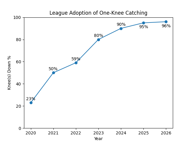
The first figure is straightforward. The percentage of pitches received from a one-knee stance rises from 23% in 2020 to 96% in 2026. What begins as a minority behavior becomes, in short order, the default condition of the position. By the end of the period, the alternative has nearly disappeared.
The second figure complicates this.
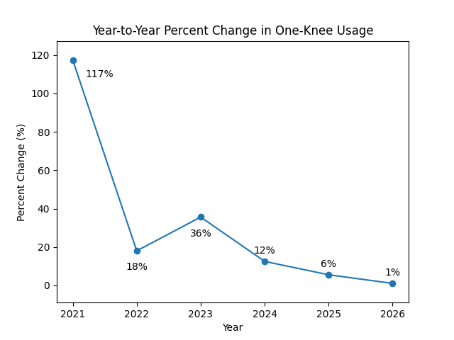
Instead of levels, it shows change. Year-to-year percentage growth in one-knee usage spikes dramatically early, then declines just as quickly. The initial jump exceeds 100%. After that, the rate of increase falls, first sharply, then gradually, until it approaches zero.
Taken together, these figures describe something more precise than simple adoption. They describe timing.
Interestingly, the decision appears to occur well before the endpoint. The first figure suggests a continuous rise through 2026. The second suggests that the meaningful shift happens earlier, closer to 2021–2023. After that, the system is no longer deciding. Decisions have been firmed up, and consolidation has taken place.
Perhaps most importantly, this pattern aligns with a familiar structure. Early adopters move aggressively, often extracting outsized value. My bet is that this is due to pitch framing. The rest of the system follows, not because the marginal gains remain large, but because the uncertainty has been resolved. Once that threshold is crossed, the behavior spreads regardless of diminishing returns.
This raises a natural question. If the rate of change collapses while the level continues to rise, what is driving the final stages of adoption?
The answer is likely institutional rather than individual. At some point, the technique ceases to be optional because the data says that it is the right thing to do. Consequently, it becomes embedded in instruction, in development, and (most importantly) in expectation. Young catchers entering the league are not choosing the one-knee stance. They are inheriting it.
This is where the first figure can mislead if taken alone. A rising line suggests ongoing discovery. The second figure suggests the opposite. Discovery is front-loaded. What follows is replication.
There is also a subtle implication for evaluation. If most of the informational gain occurs early, then later adopters are operating in a different environment. They are not testing a hypothesis. They are implementing a standard. Any performance differences observed in the later years must therefore be interpreted within a system that has already converged.
That convergence is the quiet endpoint of the process. By 2025 and 2026, the rate of change is minimal. Not because the idea has failed, but because it is clearly the right thing to do. The system has reached equilibrium.
And so, the two figures resolve into a single observation. The transformation of catching technique did not take six years; it took two or three.
Now comes the surprising part. I wondered which knee should be dropped. I know all the catchers are right-handed, so handedness is not a consideration. Fortunately, I found raw data on this. Take a look at the following figure. I find it fascinating.
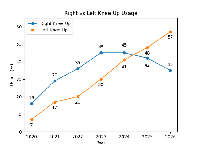
The figure reveals a subtle but meaningful asymmetry in how the one-knee stance has been adopted. Early in the period, the right-knee-up configuration is more common, but over time, the balance shifts decisively toward the left-knee-up orientation. By 2026, the split is no longer close, with the left-knee-up approach clearly dominant. Interestingly, this suggests that the evolution of the stance is not simply about going to one knee, but about settling into a preferred directional setup. The change appears gradual rather than abrupt, implying that once the broader adoption decision was made, the league continued to refine how the stance is executed rather than whether it should be used at all.
How about that? As of now, I have no idea why the preference shifted. The only thing I know is that it certainly was data-driven. My best guess is that it has something to do with giving the umpire a certain perspective when pitches are being framed. That look being the one the catcher wants the ump to have.
I am open to ideas. If you like, let me know what you think in the comments. This post certainly is fodder for a spirited discussion.
![]()
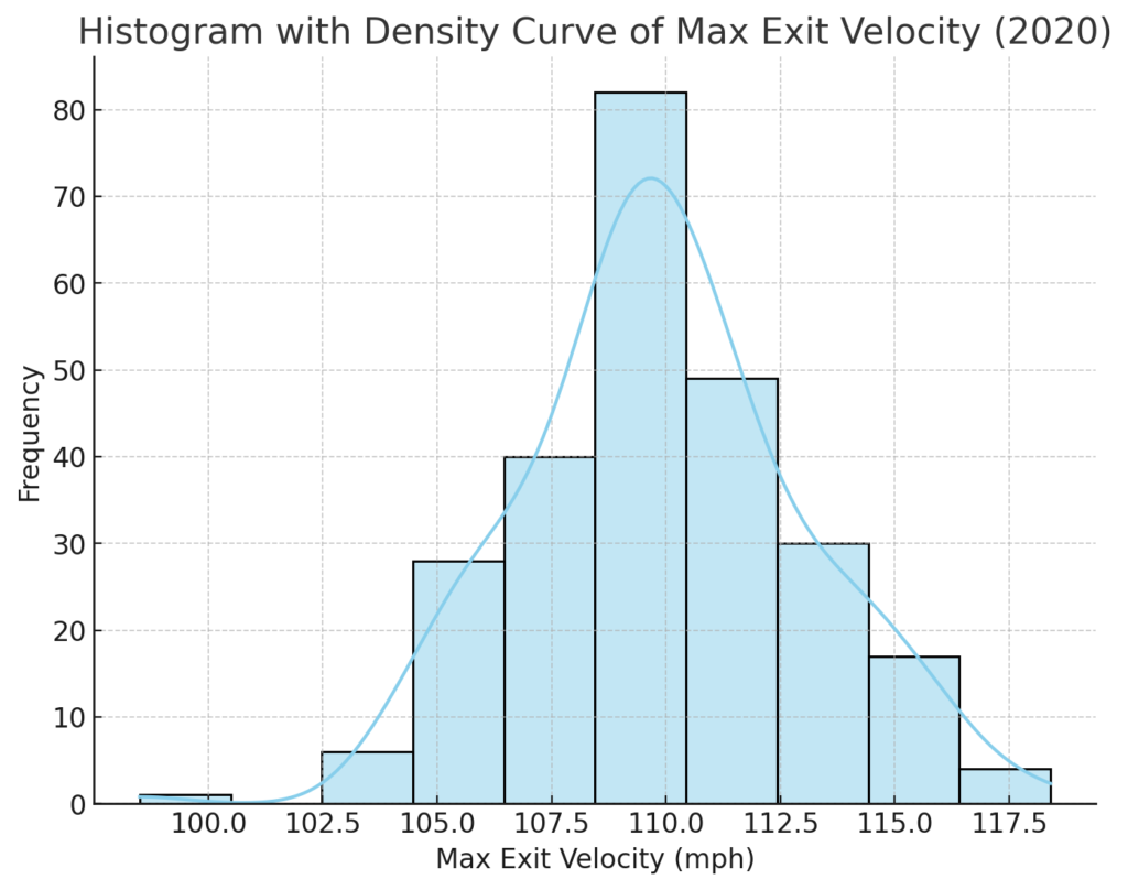
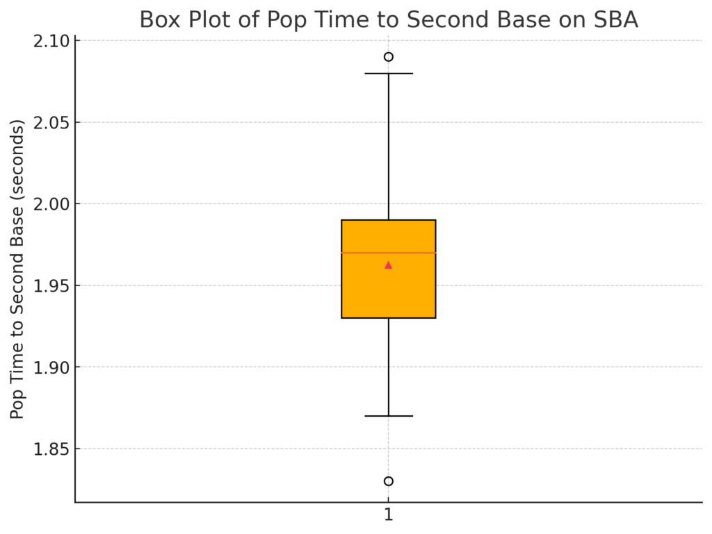
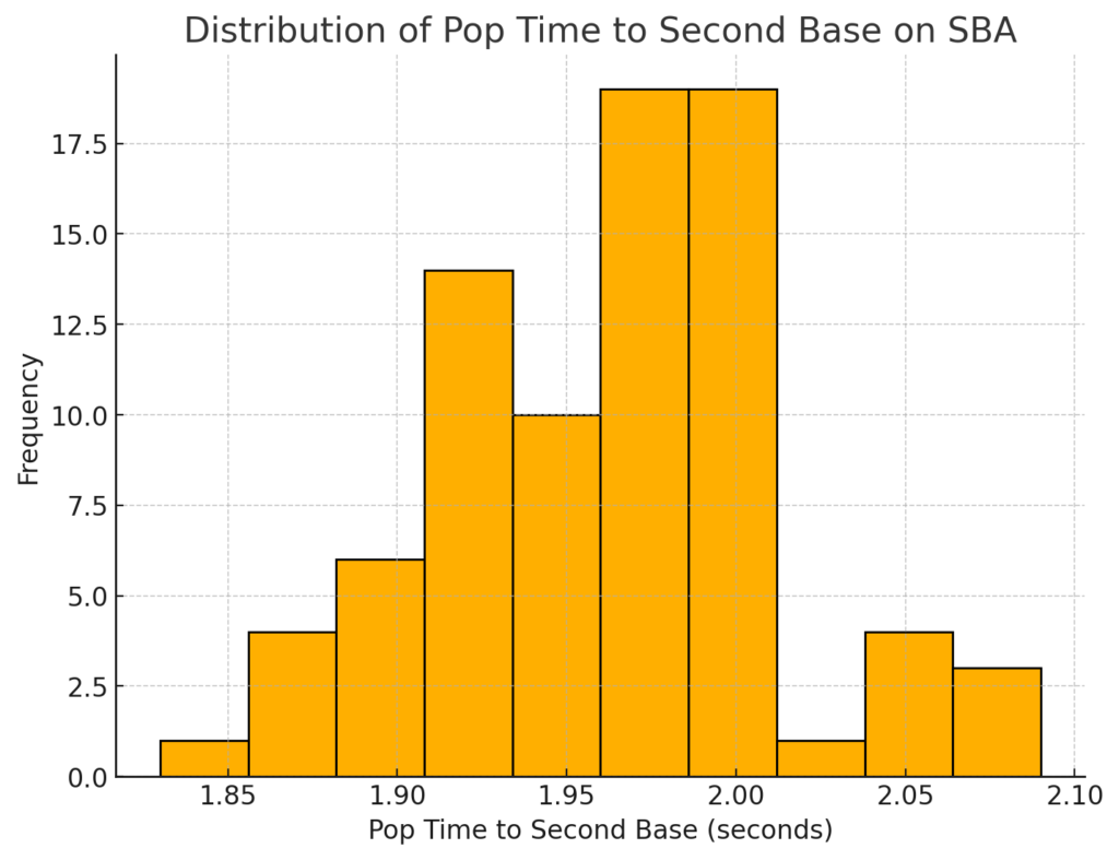 The histogram shows that most
 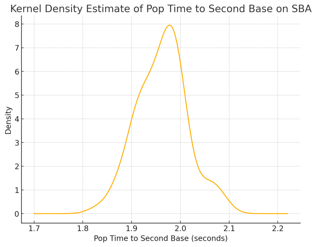 The KDE plot highlights the peak of Pop Times around 1.95 seconds, confirming that most catchers perform near this time. The data skews slightly to the right, indicating that a few catchers have slower pop times exceeding 2.0 seconds, but most fall below this threshold.
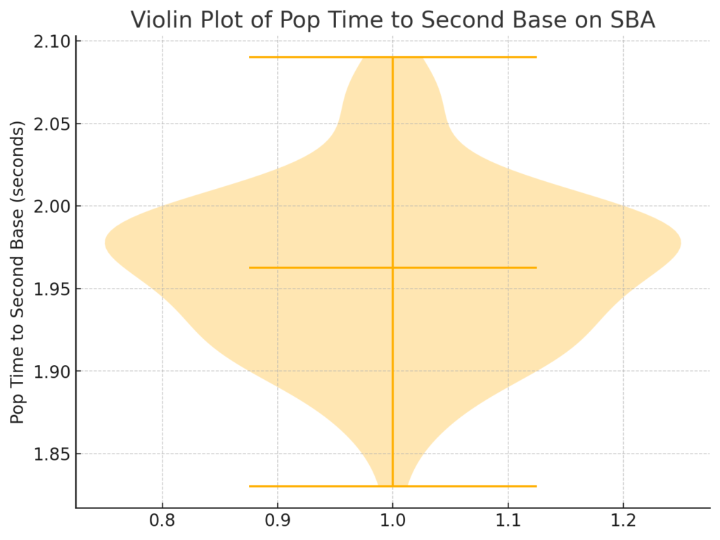 The violin plot shows that most catchers fall within a narrow range of 1.90 to 2.00 seconds. The distribution is dense around 1.95 seconds, with fewer catchers having significantly faster or slower times. This plot also highlights that catchers like J.T. Realmuto are outliers, excelling well beyond the typical range.