How Many Pitching Statistics Do We Really Need?
Correlation, Redundancy, and the Search for Independent Information in Baseball’s Pitching Metrics
Baseball has no shortage of pitching statistics.
ERA is still with us. So is WHIP. But they now share the stage with FIP, xFIP, SIERA, K-BB%, WAR, BABIP, ground-ball percentage, strikeout percentage, walk percentage, home-run rate, and an expanding collection of increasingly specialized measures.
That creates an interesting problem.
Are all these statistics actually telling us different things?
Or have we created many different ways of describing the same underlying pitching abilities?
The question became especially interesting after my study of WHIP. WHIP was very strongly associated with same-season ERA, but it was considerably weaker at predicting ERA one year later. FIP, xFIP, SIERA, and K-BB% all performed better as forward-looking measures.
That suggested a different question.
Perhaps we should stop asking which statistic is “best.”
Instead, we should ask:
How much independent information does each statistic actually contain?
That is the question I investigate here.
The Data
I used the same season-level FanGraphs dataset covering 2002 through 2025.
The data include season, innings pitched, ERA, FIP, xFIP, WAR, BABIP, home-run rate, and related pitching measures. A separate rate-statistics export includes WHIP, K%, BB%, K-BB%, ERA-, FIP-, xFIP-, FIP, xFIP, and SIERA. The batted-ball data add ground-ball percentage and related contact measures.
As in the WHIP study, I required at least 100 innings in a season:
IP_{i,y} \geq 100That produced 1,699 qualifying pitcher-seasons.
For the predictive analysis, a pitcher had to reach 100 innings in consecutive seasons:
IP_{i,y} \geq 100 \quad \text{and} \quad IP_{i,y+1} \geq 100That left 927 consecutive-season pairs involving 299 different pitchers.
Because no pitcher reached 100 innings during the shortened 2020 season, that year naturally drops out of the consecutive-season analysis.
The Metrics
The main study included:
ERA, WHIP, FIP, xFIP, SIERA, K%, BB%, K-BB%, HR/9, BABIP, GB%, and WAR.
Some of these variables are obviously related.
One relationship is exact:
\mathrm{K\!-\!BB\%} = K\% - BB\%This simple equation illustrates the broader issue surprisingly well.
K%, BB%, and K-BB% may occupy three separate columns on a leaderboard, but they do not represent three independent pieces of information.
K-BB% is constructed directly from the other two.
The relationships among FIP, xFIP, SIERA, ERA, WHIP, and the underlying pitching rates are more complicated.
But the same basic problem remains.
Different names do not necessarily mean different information.
First Look: The Correlation Matrix
The natural place to begin is with Pearson correlation.
Rather than displaying the variables in an arbitrary order, I used hierarchical clustering to place statistics with similar correlation structures near one another.
Figure 1. Correlation Structure of Major Pitching Metrics
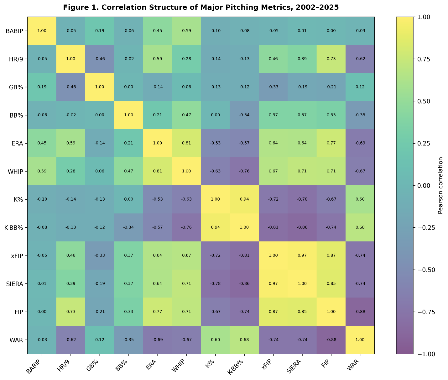
Several relationships immediately stand out.
| Metrics | Correlation |
|---|---|
| xFIP and SIERA | 0.970 |
| K% and K-BB% | 0.939 |
| FIP and WAR | -0.885 |
| FIP and xFIP | 0.873 |
| SIERA and K-BB% | -0.858 |
| FIP and SIERA | 0.854 |
| ERA and WHIP | 0.811 |
The relationship between xFIP and SIERA is extraordinary.
Their correlation is approximately:
r_{\mathrm{xFIP},\mathrm{SIERA}} = 0.970Squaring that correlation gives:
R^2 = (0.970)^2 \approx 0.941So roughly 94 percent of their observed variation is shared in a simple linear sense.
That does not make xFIP and SIERA identical. They are calculated differently and emphasize somewhat different aspects of pitching.
But statistically, they move together to an extraordinary degree.
ERA and WHIP tell a similar, though less extreme, story. Their same-season correlation is approximately 0.81.
WHIP and ERA look like different statistics.
In practice, they often move together.
Correlation Is Only the Beginning
Pairwise correlation cannot tell us everything.
A statistic may have only moderate correlations with several individual variables while still being highly predictable from all of them collectively.
This matters enormously in regression analysis.
Suppose we try to predict one variable using all the others. If that variable can already be reconstructed very accurately, then adding it to a large regression may provide very little truly new information.
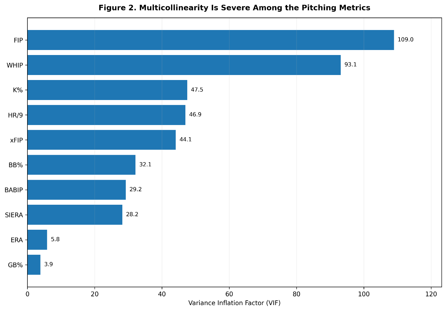
A standard way to investigate this is the Variance Inflation Factor:
\mathrm{VIF}_j = \frac{ 1 }{ 1-R_j^2 }Here, R_j^2 measures how well predictor (j) can itself be predicted by the other predictors.
A VIF near 1 suggests relatively little redundancy.
As VIF increases, multicollinearity becomes more serious.
I excluded K-BB% from this particular calculation because K%, BB%, and K-BB% have an exact mathematical dependency.
The remaining results were striking.
Figure 2. Multicollinearity Among the Pitching Metrics
| Metric | VIF |
|---|---|
| FIP | 109.0 |
| WHIP | 93.1 |
| K% | 47.5 |
| HR/9 | 46.9 |
| xFIP | 44.1 |
| BB% | 32.1 |
| BABIP | 29.2 |
| SIERA | 28.2 |
| ERA | 5.8 |
| GB% | 3.9 |
These values are enormous.
But they should not be interpreted as evidence that FIP, WHIP, or SIERA are bad statistics.
That is not what VIF measures.
The result, instead, shows that combining all these variables into a single regression equation creates extreme redundancy.
Several predictors are trying to explain the same underlying variation.
That will matter shortly.
What Should We Predict?
A statistic can look extremely impressive when it is asked to explain something happening in the same season.
Prediction is harder.
So, as in the WHIP study, I used next-season ERA as the principal target.
The general idea is:
\widehat{\mathrm{ERA}}_{i,y+1} = \beta_0 + \sum_{j=1}^{p} \beta_j z_{i,y,j}where the predictors come from year (y), while the target is ERA in year (y+1).
The predictors were standardized:
z_{i,y,j} = \frac{ x_{i,y,j} - \overline{x}_{j} }{ s_j }Standardization allows coefficients from variables measured on very different numerical scales to be compared more sensibly.
More importantly, I did not simply fit the models and report their in-sample (R2).
I used leave-one-season-out cross-validation.
One season was withheld.
The model was trained using all the other seasons.
Then it had to predict the observations belonging to the season it had not seen.
The procedure was repeated across the available seasons.
That creates a much more demanding test.
Which Single Metric Predicts Best?
Before constructing complicated regression models, it makes sense to give each statistic a chance by itself.
Figure 3. Which Single Metric Best Predicts Next-Season ERA?
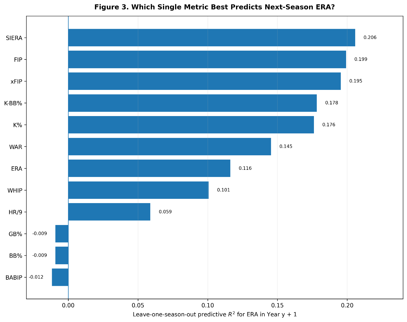
The results were:
| Predictor in year (y) | Predictive (R^2) for ERA in (y+1) |
|---|---|
| SIERA | 0.206 |
| FIP | 0.199 |
| xFIP | 0.195 |
| K-BB% | 0.178 |
| K% | 0.176 |
| WAR | 0.145 |
| ERA | 0.116 |
| WHIP | 0.101 |
| HR/9 | 0.059 |
| GB% | -0.009 |
| BB% | -0.009 |
| BABIP | -0.012 |
SIERA wins.
But only narrowly.
FIP and xFIP are very close behind it.
That is exactly what we might expect from the correlation matrix. If several statistics contain much of the same information, their predictive performance should often be similar.
K-BB% may be the most impressive result in the table.
It is remarkably simple:
\mathrm{K\!-\!BB\%} = K\% - BB\%Yet its predictive (R2) reaches approximately 0.178.
That is not far behind FIP, xFIP, and SIERA.
BABIP performs particularly poorly. Its cross-validated (R2) is slightly negative.
A negative predictive (R2) does not mean that higher BABIP magically predicts lower ERA.
It means something simpler.
For this particular prediction problem, the fitted BABIP model performs slightly worse than simply predicting the average ERA.
What Happens If We Put Everything Into One Regression?
Here is where things become interesting.
I constructed a full ordinary least-squares regression containing:
ERA, WHIP, FIP, xFIP, SIERA, K%, BB%, HR/9, BABIP, and GB%.
K-BB% was omitted because including K%, BB%, and K-BB% together would introduce exact linear dependency.
The model then produced something strange.
The standardized coefficient for WHIP was approximately:
\beta_{\mathrm{WHIP}} \approx -0.389Taken literally, that would imply that a higher WHIP predicts a lower future ERA, once the other statistics are held constant.
That is not a sensible baseball interpretation.
It is a multicollinearity problem.
Figure 4. OLS, Ridge, and LASSO Coefficients
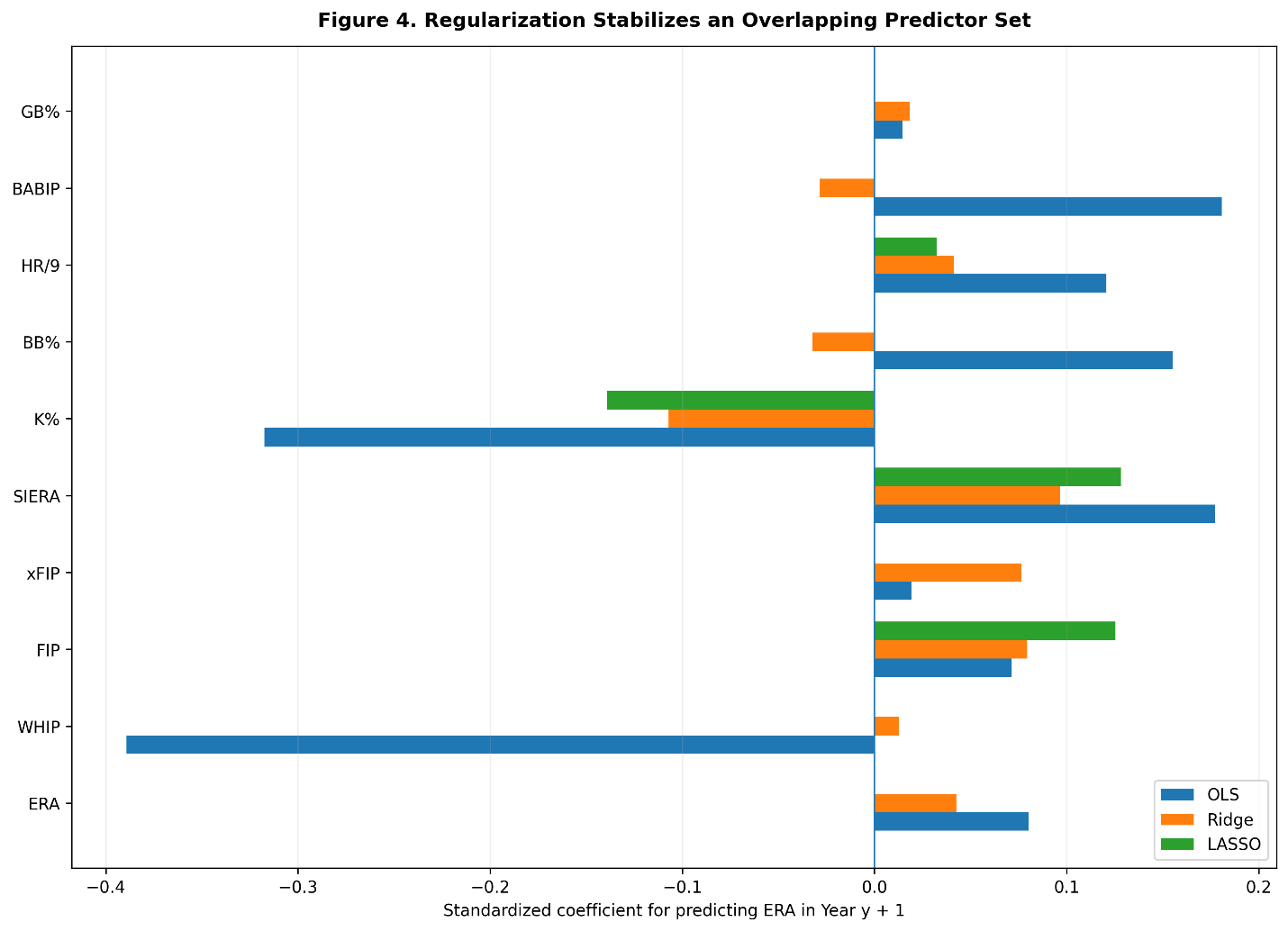
Ordinary least squares tries to divide explanatory credit among variables that contain overlapping information.
That can make individual coefficients unstable.
One variable gets a large positive coefficient.
Another highly related variable gets a negative coefficient.
A small change in the sample can alter them again.
The overall model can still predict reasonably well.
The individual coefficients, however, become difficult to interpret.
This is exactly why simply adding every available baseball statistic to a regression is not necessarily a good idea.
More variables do not automatically produce more knowledge.
Sometimes they produce more confusion.
Ridge Regression
Ridge regression offers one solution.
Rather than allowing coefficients to become arbitrarily large, Ridge penalizes them:
\min_{\beta} \left[ \sum_{i=1}^{n} \left( y_i-\widehat{y}_i \right)^2 + \lambda \sum_{j=1}^{p} \beta_j^2 \right]The tuning parameter (lambda) determines how strongly the coefficients are shrunk toward zero.
When the predictors contain large amounts of overlapping information, this can make the model considerably more stable.
That is exactly what happened.
Under ordinary least squares, the standardized WHIP coefficient was approximately -0.389.
Under Ridge regression, it became approximately:
\beta_{\mathrm{WHIP,Ridge}} \approx 0.013Essentially zero.
That is an important result.
The model is not saying WHIP is useless.
It is saying:
Once all the other pitching information is already known, WHIP contributes very little additional information about next-season ERA.
That is a very different statement.
LASSO: Let the Model Throw Statistics Away
LASSO takes the regularization idea further.
Instead of penalizing squared coefficients, it penalizes their absolute values:
\min_{\beta} \left[ \sum_{i=1}^{n} \left( y_i-\widehat{y}_i \right)^2 + \lambda \sum_{j=1}^{p} \left| \beta_j \right| \right]This has an interesting consequence.
LASSO can set some coefficients exactly to zero.
That turns our original question into an empirical experiment.
Give the model all these pitching statistics.
Then ask:
Which ones does it decide it does not need?
In the full-sample fit using the cross-validated penalty, LASSO retained four nonzero predictors:
FIP
SIERA
K%
HR/9
ERA went to zero.
WHIP went to zero.
xFIP went to zero.
BB%, BABIP, and GB% went to zero.
This does not mean those discarded statistics contain no useful baseball information.
It means that, for predicting next-season ERA after the retained variables were already available, their additional contribution was small enough that LASSO discarded them.
That is precisely the kind of redundancy we set out to investigate.
How Stable Was LASSO’s Decision?
A single LASSO fit is useful, but correlated predictors can substitute for one another.
So I also examined how often each statistic survived across the outer cross-validation folds.
Figure 5. Which Metrics Does LASSO Keep?
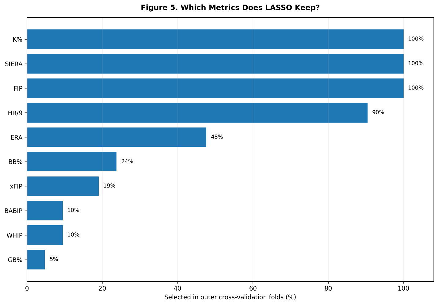
The approximate selection frequencies were:
| Metric | Selected |
|---|---|
| FIP | 100% |
| SIERA | 100% |
| K% | 100% |
| HR/9 | 90% |
| ERA | 48% |
| BB% | 24% |
| xFIP | 19% |
| WHIP | 10% |
| BABIP | 10% |
| GB% | 5% |
Three statistics survived every time:
FIP, SIERA, and K%.
HR/9 survived in approximately 90 percent of the folds.
WHIP survived only about 10 percent of the time.
That is particularly interesting after the previous WHIP study.
WHIP is very good at describing current run prevention.
Yet once the regression already knows FIP, SIERA, strikeout rate, home-run rate, and the other variables, WHIP rarely contains enough unique predictive information to survive LASSO.
That is not a contradiction.
It is the distinction between useful information and unique information.
Does the Giant Model Actually Predict Better?
Now we arrive at the question that matters most.
Perhaps all this redundancy does not matter if the large model predicts much better.
Does it?
Figure 6. More Metrics Help, but Only a Little
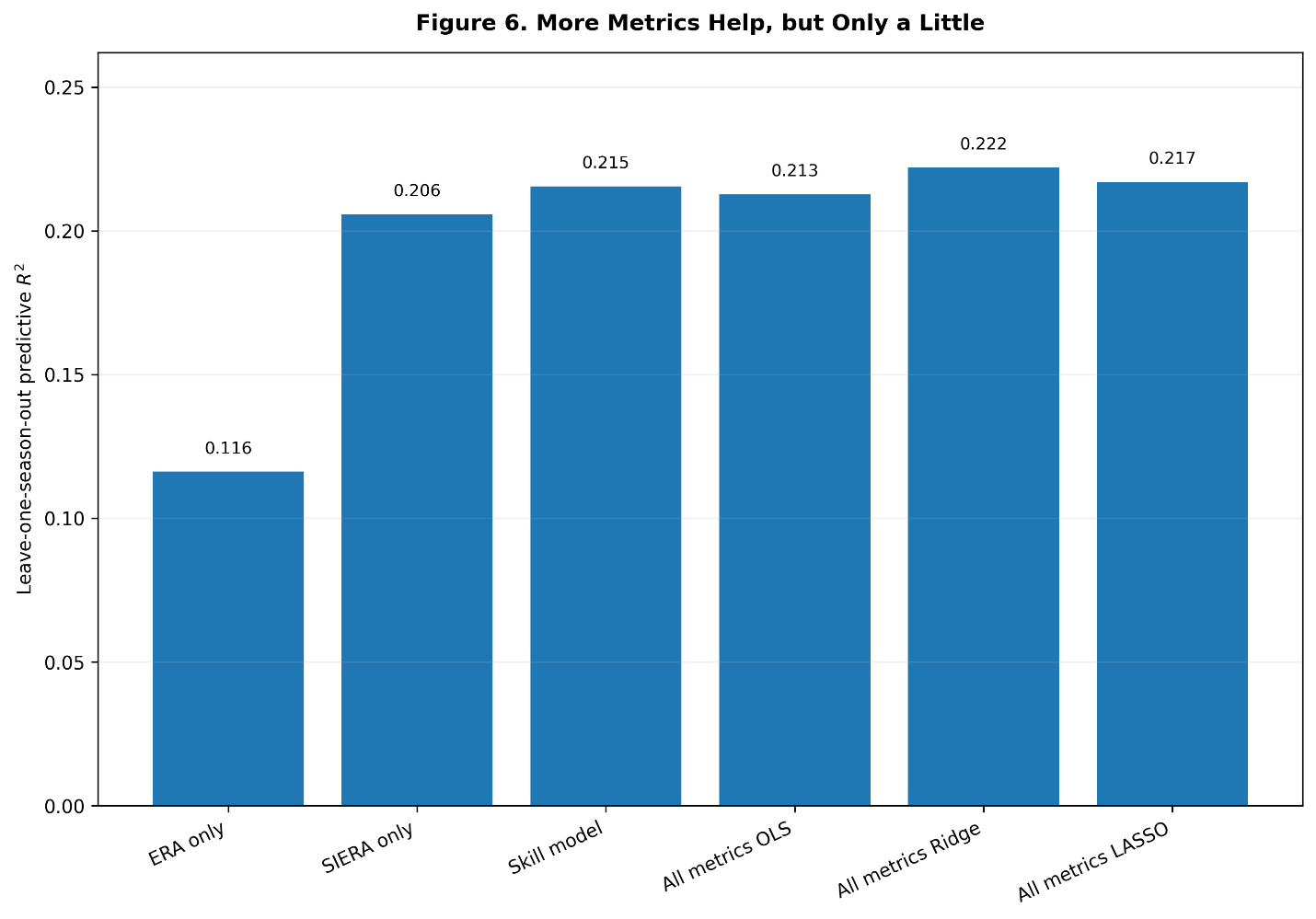
The cross-validated results were:
| Model | Predictive (R^2) |
|---|---|
| ERA only | 0.116 |
| SIERA only | 0.206 |
| Five-skill model | 0.215 |
| All metrics, OLS | 0.213 |
| All metrics, Ridge | 0.222 |
| All metrics, LASSO | 0.217 |
The five-skill model used K%, BB%, HR/9, BABIP, and GB%.
The best model was the full Ridge regression.
Its predictive (R2) was approximately:
R^2_{\mathrm{Ridge}} = 0.222SIERA alone produced:
R^2_{\mathrm{SIERA}} = 0.206The improvement was therefore:
\Delta R^2 = 0.222 - 0.206 = 0.016Just 1.6 percentage points.
The RMSE tells essentially the same story.
SIERA alone produced an RMSE of about 0.737 ERA runs.
The full Ridge model reduced that to approximately 0.729.
The larger model is better.
But only a little.
That may be one of the most important results in the study.
We gave the model a large collection of modern pitching statistics.
Most of the additional information barely moved the prediction.
Once We Know SIERA, What Else Helps?
This provides another way to look at redundancy.
Start with SIERA, the strongest individual predictor.
Then add other statistics one at a time.
Figure 7. Once We Know SIERA, Most Extra Metrics Add Very Little
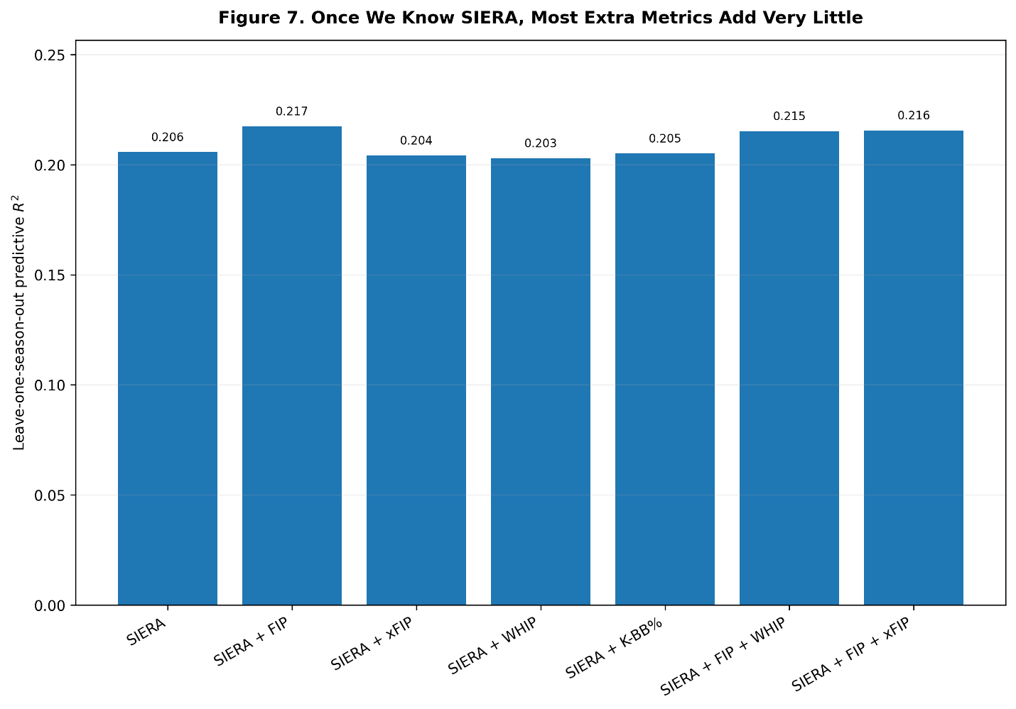
SIERA alone:
R^2 = 0.206Add FIP and the result improves to approximately:
R^2 = 0.217That is a genuine, although modest, improvement.
Add xFIP to SIERA and predictive performance actually slips slightly, to approximately 0.204.
Add WHIP and it falls to roughly 0.203.
Adding K-BB% changes almost nothing.
Even combining SIERA, FIP, and xFIP reaches only about 0.216.
This is a remarkably clean demonstration of statistical redundancy.
Three statistics are not necessarily three times as informative as one.
Sometimes the second statistic is largely repeating the first.
The third repeats them both.
Why xFIP and SIERA Are a Good Example
Consider again:
r_{\mathrm{xFIP},\mathrm{SIERA}} = 0.970If two statistics move almost perfectly together, there is simply not much room for one to add entirely new predictive information after the other is already known.
They can still differ conceptually.
Their formulas can still have different purposes.
Their disagreements can even be analytically useful.
But conceptual difference does not guarantee statistical independence.
That distinction is central to this study.
What About WAR?
ERA is only one possible definition of future pitching success.
So I repeated the regression analysis using next-season WAR as the target.
Current WAR itself was the strongest individual predictor:
R^2_{\mathrm{WAR}_y,\mathrm{WAR}_{y+1}} \approx 0.336SIERA reached approximately 0.252.
FIP reached about 0.243.
xFIP was around 0.235.
WHIP was considerably weaker at approximately 0.125.
Figure 8. Predicting Next-Season WAR
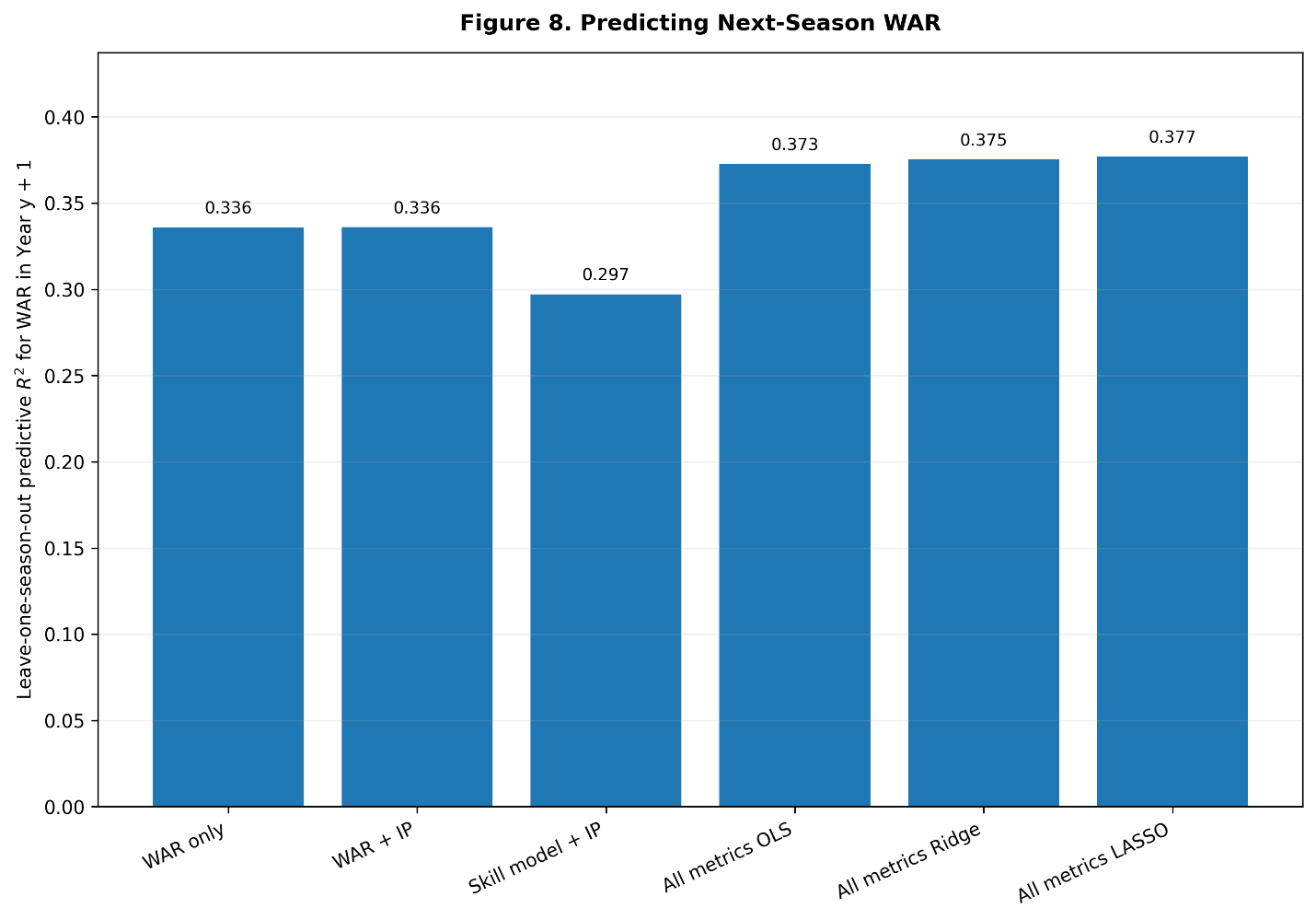
The multivariable models produced:
| Model | Predictive (R2) |
|---|---|
| WAR only | 0.336 |
| WAR + IP | 0.336 |
| Skill model + IP | 0.297 |
| All metrics OLS | 0.373 |
| All metrics Ridge | 0.375 |
| All metrics LASSO | 0.377 |
Here the large models add somewhat more information.
The best LASSO model improves predictive (R2) from roughly 0.336 using current WAR alone to approximately 0.377.
That is a more noticeable gain than we observed when predicting ERA.
Still, the central lesson remains.
Adding many statistics helps.
But the improvement is nowhere near proportional to the number of variables added.
The Strange WHIP Coefficient Revisited
The negative WHIP coefficient in the ordinary regression is worth returning to because it demonstrates an important statistical point.
WHIP by itself predicts future ERA in the expected direction.
Higher WHIP is associated with higher future ERA.
But once we tell an ordinary regression to hold ERA, FIP, xFIP, SIERA, K%, BB%, HR/9, BABIP, and GB% constant, the WHIP coefficient becomes negative.
Those are two very different questions.
The simple regression asks:
What happens to future ERA when WHIP changes?
The giant multiple regression asks:
What happens when WHIP changes while an enormous collection of closely related pitching statistics somehow remains fixed?
That second scenario may have very little resemblance to an actual pitcher.
The variables are too interconnected.
OLS nevertheless tries to divide the shared information among them.
The resulting coefficient is mathematically legitimate.
Its baseball interpretation is questionable.
Ridge responds by shrinking the WHIP coefficient almost to zero.
LASSO simply removes WHIP.
Both approaches give us a more sensible picture of what the data are saying.
How Many Statistics Do We Really Need?
There is no universal answer.
It depends on the question.
If I want to know how successfully a pitcher kept runners off base, WHIP is excellent.
If I want to know how many earned runs he actually allowed, ERA tells me exactly that.
If I want a simple forward-looking estimate of next-season ERA, SIERA performed best among the individual metrics examined here.
If I want to squeeze out every additional bit of predictive accuracy, a regularized multivariable model performs somewhat better.
But the key word is somewhat.
Going from SIERA alone to a ten-variable Ridge regression improved predictive (R2) from about 0.206 to 0.222.
The sophisticated model wins.
Barely.
The Bigger Lesson
A modern baseball leaderboard can create an illusion of enormous amounts of independent information.
Twenty columns look like twenty facts.
Statistically, that may not be true.
Strikeout ability appears directly in K%.
It appears again in K-BB%.
It also enters FIP, xFIP, and SIERA.
Walks do the same.
Home runs affect FIP and other estimators.
BABIP influences hit-based measures.
ERA and WHIP share the consequences of allowing baserunners.
The columns multiply faster than the underlying baseball phenomena.
That is not a criticism of advanced statistics.
Different metrics were created to answer different questions. They emphasize different aspects of performance. They make different assumptions. They may be useful in different contexts.
The mistake would be assuming that because two statistics have different names, they must contain completely different information.
They often do not.
Conclusion
The original question was simple:
How many pitching statistics do we really need?
The answer is more interesting than I expected.
Many pitching metrics are strongly correlated.
Some are extraordinarily correlated.
xFIP and SIERA correlate at approximately 0.97. ERA and WHIP correlate at about 0.81. FIP, xFIP, SIERA, strikeout measures, walk measures, and home-run measures overlap so heavily that placing all of them in the same ordinary regression produces severe multicollinearity.
The VIF analysis shows the problem.
The unstable OLS coefficients make it visible.
Ridge regression controls it.
LASSO begins throwing redundant statistics away.
And the predictive results show just how little we lose by simplifying.
SIERA alone explains about 20.6 percent of next-season ERA variation under leave-one-season-out prediction.
A full ten-variable Ridge model improves that to approximately 22.2 percent.
Ten statistics are better than one.
But not by much.
That may be the most important conclusion.
The goal should not be to collect the largest possible number of metrics.
It should be to identify statistics that represent genuinely different dimensions of pitching.
After that point, we increasingly begin measuring the same underlying abilities again.
And again.
Just under different names.