The Face of the Data: Herman Chernoff, SYSTAT, and the Art of Seeing Statistics

I have always had a particular affection for Chernoff Faces.

Decades ago, when I was using SYSTAT for statistical analysis, I would occasionally generate these peculiar little icons. Some smiled. Others frowned. A few looked surprised, suspicious, or vaguely irritated. They resembled cartoon characters, but not in the ordinary sense. They were data.

Every feature could represent a numerical measurement: the width of a face, the size of the eyes, the angle of the eyebrows, or the curvature of a mouth. A table of multivariate observations became a small crowd of expressive characters. I thought the idea was brilliant then. I still do.

What if one of our best instruments for recognizing patterns was something the human brain already knew how to read: a face?

A statistician gives the data a face

In 1973, Herman Chernoff published “The Use of Faces to Represent Points in k-Dimensional Space Graphically” in the Journal of the American Statistical Association. His proposal appears both practical and wonderfully eccentric. Human beings are skilled at distinguishing faces, so perhaps facial features could carry several dimensions of numerical information at once.

Chernoff’s original design allowed as many as eighteen numerical features to be encoded. That does not mean viewers can reliably recover eighteen numbers from a glance. It means a single observation can be rendered as an object whose shape varies systematically with a collection of measurements.

The distinction is critical. Representation is not the same as interpretation. An image can contain information without making all of that information equally accessible.

From a baseball season to a face

To investigate the idea, I returned to familiar territory: baseball. I used an existing Lahman-derived offensive dataset covering 1954 through 2025 and selected twenty notable player-seasons, one season per player, using a five-variable offensive score. This is a deliberately selected comparison set, not a random sample of all MLB seasons or a definitive ranking of the greatest twenty seasons.

Five measurements went into the experiment: on-base percentage (OBP), isolated power (ISO), walks per plate appearance (BB/PA), strikeouts per plate appearance (SO/PA), and net stolen bases per plate appearance (NetSB/PA). Strikeout rate was reverse-coded so that the corresponding standardized measure rewarded fewer strikeouts. The first four measures emphasize reaching base, power, and discipline; the fifth features a base-running dimension.

My broader Model C uses seven offensive variables. This experiment uses five because those are the measures available in the comparison dataset. Runs per plate appearance and RBI per plate appearance are not included in this particular set of faces.

We can begin by describing each season as a 5-dimensional vector:

\mathbf{x}_i = (x_{i1},x_{i2},x_{i3},x_{i4},x_{i5})

Because the variables have different ranges, we standardize them before building a composite:

z_{ij} = \frac{x_{ij}-\bar{x}_j}{s_j}

The resulting score is the sum of the five appropriately oriented standardized measures:

\begin{aligned}\mathrm{Score5}_i ={}& z_{\mathrm{OBP},i}+z_{\mathrm{ISO},i}\\&+z_{\mathrm{BB/PA},i}+z_{\mathrm{LowSO},i}\\&+z_{\mathrm{NetSB/PA},i}\end{aligned}

Standardization was carried out in the historical source analysis; the Chernoff experiment uses the resulting player-season values. The purpose of the score is to select a diverse set of outstanding performances, not to settle which player was best.

Same numbers, different faces

The first experiment is simple. Draw each of the twenty seasons as a face, assigning each offensive variable to one visual feature. Then draw the same twenty seasons again, changing the assignments while leaving every numerical observation untouched.

In one mapping, OBP might control mouth curvature while another variable changes eye size. In the second mapping, the same variables are redirected to different features. Facial shapes should therefore change, although the players’ numbers and their underlying multivariate relationships do not.

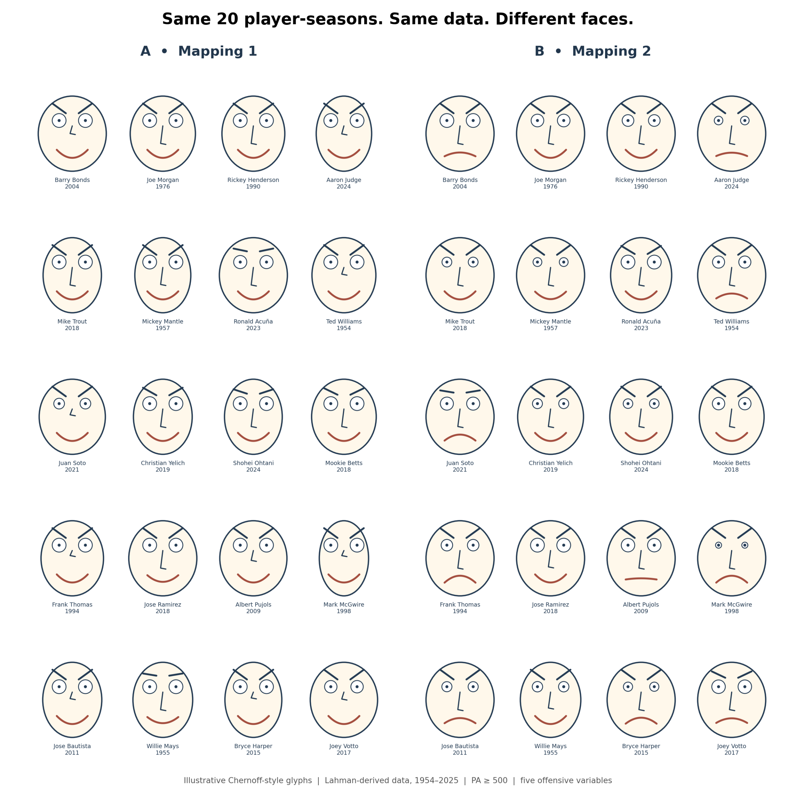
Figure 1. The same 20 player-seasons under two assignments of numerical variables to facial features. The data do not change, but the expressions do.

Barry Bonds’s 2004 season is especially memorable. In the first mapping, his face smiles. In the second, it frowns. Nothing happened to his on-base percentage or his power. Only the drawing rules changed.

This is both the charm and the danger of Chernoff Faces. A smiling face appears positive, even when the statistical variable driving the smile may have no positive emotional meaning at all. A face with an ominous expression may represent a remarkable performance.

Why a face can mislead

We are not equally sensitive to every feature of a face. Mouth curvature and eye size can dominate a first impression, while a comparably large change in nose length may be barely noticed. Therefore, a variable mapped to the mouth can have more perceptual influence than an equally important variable mapped to a subtler feature.

Chernoff and M. Haseeb Rizvi studied a version of this problem in 1975. Their work showed that reassigning variables to facial characteristics could affect classification errors. The issue is not simply philosophical. Choice of visual encoding can change how easily observers classify the same observations.

Figure 2 concentrates on selected players so that this transformation is easier to see.

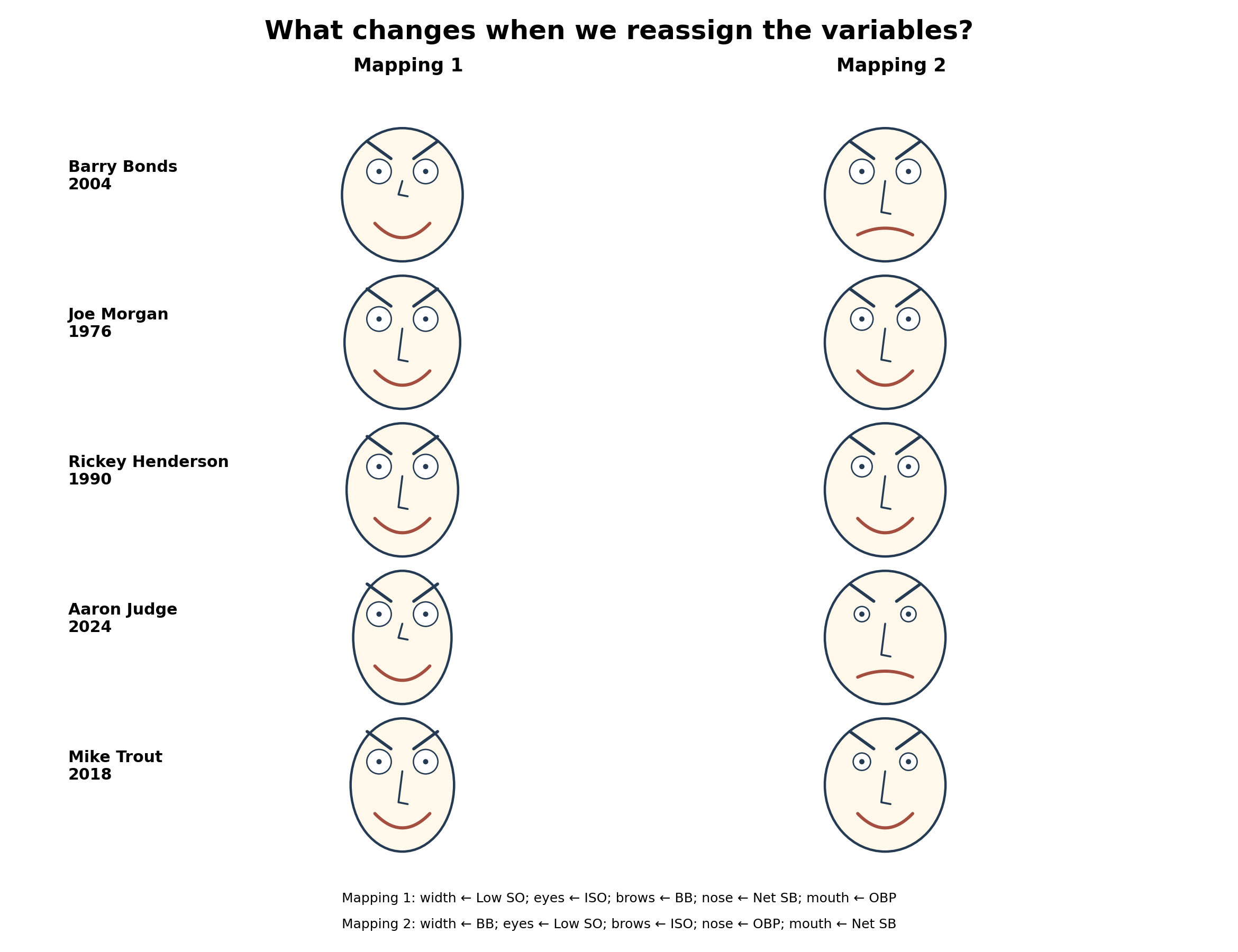
Figure 2. Selected player-seasons displayed with alternative facial mappings. These are illustrative Chernoff-style glyphs, not measurements of player personality or emotion.

There is an important asymmetry here. The underlying distance between any two observations stays fixed. But the viewer’s impression of similarity may move with the mapping. A graphical convention has introduced a psychological variable into the interpretation of a mathematical relationship.

Every statistical graphic involves choices. A histogram depends on bin width, a heat map on its palette, and a scatterplot on its axes. Chernoff Faces make that dependence unusually visible, because our response to faces is immediate and difficult to suppress.

Chernoff meets Tukey

John Tukey emphasized that exploratory data analysis starts with discovering structure, not simply confirming a predetermined hypothesis. On that view, Chernoff Faces make sense. They are not a statistical test and do not supply a confidence interval. They ask us to notice something unexpected and then check it by more rigorous methods.

Imagine two player-seasons with nearly identical composite scores. One may derive its advantage from power and walks, the other from contact and base running. Their total scores may conceal substantially different offensive profiles. A set of faces could make that contrast apparent before we examine the component measurements.

The key word is “might.” A face that attracts our attention is not evidence of a genuine cluster or outlier. It is a reason to look for one.

What if the faces lived inside a PCA?

I also tried a hybrid: using a principal component analysis to position the player-seasons while drawing Chernoff Faces instead of ordinary dots. PCA finds directions through the numerical data that account for as much variation as possible. The faces retain the separate measurements in their features.

For this selected sample, the first two principal components explain approximately 51.7% and 28.0% of the standardized variation, respectively, or about 79.7% together. Those percentages describe this selected set of twenty seasons, not all baseball players.

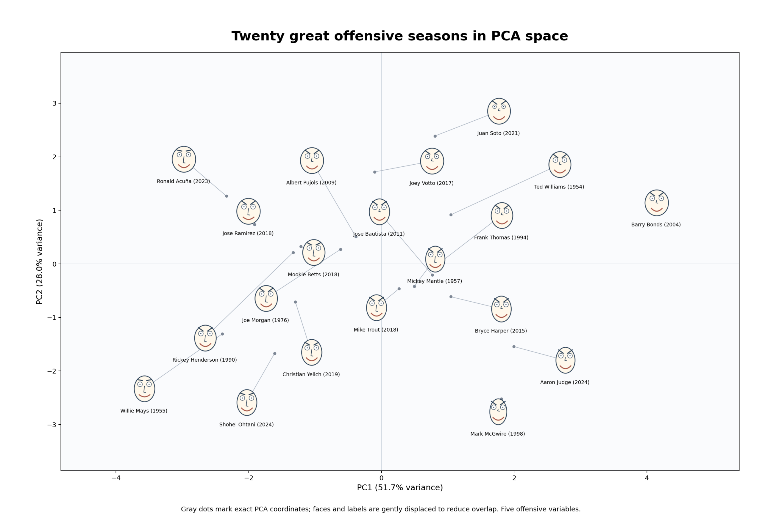
Figure 3. Chernoff-style faces over a two-component PCA display. Small markers show exact PCA positions; some faces are offset to preserve readability.

The result is intriguing. The coordinates provide a reproducible mathematical geography of offensive profiles. The faces add a visual indication of how those profiles differ. At a glance, we can ask not only which observations are near one another, but what combination of traits makes them distinctive.

We should resist reading too much into the appearance of a particular face, especially in a small, hand-selected sample. Still, as a device for generating questions, the hybrid has real appeal.

Distance is mathematical, resemblance is perceptual

Suppose we want to compare two seasons in standardized five-dimensional space. Their straight-line distance is:

d(i,j) = \sqrt{\sum_{k=1}^{5}(z_{ik}-z_{jk})^{2}}

Changing which variable controls the mouth or the eyes does not change this distance. Yet if the visual features attract different amounts of attention, the apparent resemblance between two faces can change dramatically.

We can even construct an illustrative model in which facial features receive unequal weights. In a preliminary exercise with assumed weights, the rank correlation between numerical distance and visually weighted distance was about 0.70 under one mapping and 0.59 under another. These are properties of the chosen weighting model, not results from a study of human observers. They should not be interpreted as measured perception.

The proper experiment would ask actual viewers to sort faces into groups or identify outliers, with facial assignments randomized across conditions. We could compare those responses with a distance matrix or clustering solution computed from the original set of variables. That should test the gap between statistical structure and perceived similarity rather than simply illustrate it.

Would I use Chernoff Faces today?

Certainly (I just did). Not as a replacement for regression, PCA, clustering, or conventional graphics, but as a companion to them. I would use them to provoke questions, compare profiles, and remind readers that any plot is a translation of numbers into something our senses can grasp.

I might even use them in a larger study of great offensive seasons, expanding the historical dataset to include Babe Ruth and restoring the full seven-variable Model C. But that would require rebuilding the dataset and rechecking historical comparability; our present experiment begins in 1954 and cannot legitimately include Ruth.

I remember the pleasure of producing these images in SYSTAT, back when statistical graphics were much less elaborate than they are now. Their simplicity was part of their appeal. A face could tell you where to look without pretending to tell you everything you needed to know.

More than fifty years after Chernoff’s paper, I still think this is a marvelous idea. It sits at the intersection of mathematics and perception, where many of the most interesting questions within data analysis begin.

The numbers haven’t changed; only the way we look at them has.

References

Chernoff, H. (1973). The use of faces to represent points in k-dimensional space graphically. Journal of the American Statistical Association, 68(342), 361–368.

Chernoff, H., & Rizvi, M. H. (1975). Effect on classification error of random permutations of features in representing multivariate data by faces. Journal of the American Statistical Association, 70(351), 548–554.

Tukey, J. W. (1977). Exploratory Data Analysis. Addison-Wesley.